Analytical modeling of cylindrical eddy current brakes and multi-objective optimization based on game theory

Fan, Yumeng; Yang, Guolai; Sun, Quanzhao

doi:10.21595/jve.2024.24065

Journal of Vibroengineering

Browse Journal

Submit article

Published: 31 July 2024

Check for updates

Analytical modeling of cylindrical eddy current brakes and multi-objective optimization based on game theory

Yumeng Fan¹

Guolai Yang²

Quanzhao Sun³

^{1, 2, 3}School of Mechanical Engineering, Nanjing University of Science and Technology, Nanjing, 210094, China

Corresponding Author:

Yumeng Fan

Cite the article Download PDF

Downloads 67

Abstract

With the research and development of eddy current brake (ECB), today ECBs have been applied in a variety of fields including vibration control and braking of strong impact loads.The application of a new cylindrical structure eddy current brake (ECB) for strong impact braking of large machinery has been discussed recently. Its high-speed and high-kinetic-energy braking conditions require different analytical and optimization design models and methods from what has been addressed in previous studies. For subsequent more engineering-oriented research and optimization, modeling methods are needed, as well as analysis and optimization studies for braking forces and critical speeds of interest. In this work, a magnetic equivalent circuit model is established, and the influence of eddy current induced during application is taken into account by considering it as a magnetomotive force in the model. The braking force is calculated with the MEC model and an approximate electric field cross-section method. A small prototype experiment is carried out and proves the correctness of the proposed model. Using the proposed and FEM model, parameters of the ECB are analyzed. Then, aiming at design objectives of the ECB that are somewhat competitive under this special braking condition, a multi-objective optimization model is established using the Stackelberg game strategy. An FEM model is built and assessed based on optimization results. The results indicate that the multi-objective optimization model based on the Stackelberg game is effective for the design of this ECB structure.

1. Introduction

The eddy current brake (ECB) is a new type of braking method that has developed in recent years. Different from the traditional braking device, an ECB can brake without contact, and the excitation-type ECB can also control the magnitude of the braking force. This braking method has been applied in many fields, such as heavy-duty vehicle retarders, dampers for vehicle suspension systems, tuned mass dampers for footbridges, etc., and there is also related research in the aerospace field [1-4].

There have been many ECB structures that have been researched and applied, such as axial ECB structures, hybrid excitation linear ECBs, Halbach structures, and so on [5-8]. In recent years, the ECB structures studied have mainly been of the torque type or linear type with plate structure [9, 10]. However, the ECB discussed in this paper has a cylindrical structure and is applied to large machines with strong impact loads, which have not been studied much. For the subsequent more engineering-oriented research and optimal design, modeling methods and analysis as well as multi-objective optimization studies are needed. Generally speaking, the study and analysis of the ECB requires a reliable analytical model that can predict the magnetic field and braking force. A commonly used magnetic field analytical model is called the magnetic equivalent circuit (MEC) model. However, the MEC model is most precise when it is not loaded, because it is difficult to accurately add the influence of eddy current into the model [11-13]. Through Maxwell’s equations [14, 15], a model that can simulate and predict an ECB more accurately can be obtained, but this method is complicated and computationally time-consuming and is not necessary in the preliminary design of an ECB.

The finite element model is also an effective means to study the ECB. Some researchers use the finite element method to model ECBs [16, 17], and finite element software can also be used to model and analyze ECBs. The use of finite element software to analyze ECBs does not require complex mathematical modeling, and at the same time, visual calculation results can be obtained, which can provide great convenience for analysis and research. But at the same time, finite element modeling and calculation in the software are also more time-consuming [18, 19].

After obtaining an effective ECB analysis model, the model can be used in design parameters analysis and optimization of an ECB. Some current design-related ECB studies analyzed the influence of parameters on the braking force, the values of the design parameters were selected based on the analysis, and the design of the ECB were decided by checking the braking force requirements [20-22].

The design of the permanent magnet (PM) ECB structure studied in this paper is aimed at the ECB being able to obtain greater braking force at higher speeds. To achieve this, a multi-objective optimization model [23] including two optimization objectives of high braking force and high critical speed is needed.

Recently, there have been three approaches utilized for managing these kinds of multi-objective optimization problems: weighted average optimization, non-dominated optimization, and game theory. Weighted average methods solve multi-objective optimization problems by assigning each objective function a weight and deriving a single objective optimization problem. This method needs reasonable weight decisions for the objectives [24]. Non-dominated optimization methods have been widely applied in many fields. Common algorithms for such methods, such as the non-dominated sorting genetic algorithm (NSGA-II), find non-dominated solutions by applying evolutionary algorithms with Pareto ranking [25].

Game theory is a mathematical theory and method of studying phenomena of a combat or competitive nature. Players cooperate or compete to improve their own gains in the game. Game theory has been widely used in research in fields such as finance and political science. In recent years, by transforming players into optimization objectives, some research in mechanical design has integrated the game theory method into the multi-objective optimization algorithm. Two game strategies have been introduced before, which are the Nash game strategy and the Stackelberg game strategy.

The Nash game was proposed by John Nash [26]. The two or more players in the game are assumed to know the strategy of each other, and when neither can gain any additional profit by unilaterally changing their own strategy, it can be called a Nash equilibrium. There are studies in many fields that incorporate Nash game theory into multi-objective optimization problems. For example, there are applications in machine tool spindle optimization, multi-criterion aerodynamic shape design optimization for conveyors, transonic wing shape optimization, and so on [27-29].

Unlike the Nash game, there is a leader among the players in the Stackelberg game [30], and the leader’s status is higher than the other players – the followers. Players are activated hierarchically to perform optimizations, and when the leader can no longer improve the strategy, it is considered that a Stackelberg equilibrium is reached. Li et al. applied this method to the control of parameter optimization in uncertain fuzzy systems [31]. To study the binary zero-sum Stackelberg game between missile-borne radar signals and jamming, Wang H et al. carried out two games, each with a different leader, and provided optimization solutions for radar signals and jamming signals separately [32]. The Stackelberg game strategy has also been applied in the optimization of the airfoil or the multi-airfoil [33, 34]. And to solve single-objective and two-objective aerodynamic shape optimization problems, Jing W et al. coupled the Stackelberg game strategy with the adjoint method [35].

The ECB studied in this paper intended for braking under high-speed operating conditions, i.e., it is required to perform better brake force under the speed condition needed. However, with different structure and parameter design, the critical speed of ECB reduces when the braking force is increased. That is to say, the two optimization objectives in ECB’s multi-objective optimization model are competitive under certain situation. However, braking force is still prioritized over critical speed, as well as the ECB mass that always needs to be considered. That is, the optimization objectives in this paper are conflicting to some extent, but the braking force requirement is predominant. Therefore, Stackelberg game theory is chosen in this paper as being well suited for application to optimization models.

In this paper, a new modeling approach for ECB braking force prediction model was proposed and a modeling methodology study for multi-objective optimization using a game theory approach was conducted. The main tasks and studies carried out are as follows. Firstly, this paper presents an analytical model whose MEC model considers the influence of eddy currents in the magnetic circuit by adding induced magnetomotive force. Finite element models were established, and some complicated Maxwell equations were bypassed by analyzing the finite element model. Combining it with the MEC model, a simple and fast predictive analytical model is obtained. A similar modeling approach was established and validated using the graphical method in [36], and in this paper it has been modeled using the fitting method. Secondly, through small size prototype experiments and comparing the results with the finite element model calculations, the model proposed in this paper was considered reliable and could show the influence law of different parameters on the ECB braking force, i.e., it can be directly used for the optimization of the model. Then, with this proposed model, a multi-objective optimization model for the studied ECB was established with the Stackelberg game and the proposed model, and the optimization result was verified by FEM models.

2. The linear PM ECB analysis MODEL

2.1. The structure and MEC model of the ECB

The ECB model studied in this paper is shown in Fig. 1. It is a linear ECB, but instead of an upper and lower layered structure, it adopts an inner and outer cylinder structure. To optimize the ECB model design, a reliable analysis model should be established and its design parameters analyzed. In this section, a magnetic circuit analysis model based on magnetic equivalent circuit (MEC) method will be established.

Fig. 1a) PM linear ECB and b) its partial schematic diagram (Reproduced with permission from [Analytical modeling of permanent magnet linear eddy current brake using magnetic equivalent circuit method], IOS Press, 2022)

a) PM linear ECB and b) its partial schematic diagram (Reproduced with permission from [Analytical modeling of permanent magnet linear eddy current brake using magnetic equivalent circuit method], IOS Press, 2022)

a)

b)

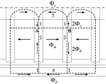
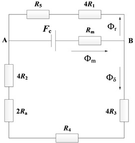
Fig. 1 demonstrates the ECB structure studied in this paper, which mainly consists of two parts: the primary part, with multiple sets of cylindrical PM and pole shoe alternately arranged on the shaft; and the secondary part, which is composed of conductor cylinder and back iron cylinder. PMs are axially magnetized, and adjacent PMs always have opposite magnetized directions. The enlarged schematic diagram of the ECB shown in Fig. 2(a) can help to see the specific size parameters. $r_{0}$ is the radius of the shaft; $d_{m}$ , $r_{p m}$ are the axial thickness and external radius of PMs; $d_{s}$ , $r_{i p}$ are the axial thickness and external radius of pole shoes; $r_{i}$ , $r_{b}$ are internal radius of the inner cylinder conductor and back iron.

In addition, $d$ is the pole pitch; $h_{p m}$ in the figure is the value of the outer diameter of the PM minus the inner diameter; $h_{d}$ in the figure is the value of the outer diameter of pole shoe minus the outer diameter of PM. And $h_{a}$ and $h_{i}$ are the radial thickness of air gap and cylinder conductor; $r_{e b}$ is the external radius of back iron.

The ECB structure is simplified to a two-dimensional axisymmetric model. In order to perform MEC analysis and model building, assumptions need to be given. There is no magnetic saturation phenomenon considered in the ECB model, and the relative recoil permeability of PM is assumed to be constant. In the ECB model discussed in this paper, the operating point of the PMs generally will not exceed the linear stage of the demagnetization curve, so the PMs in the model is assumed to be linearly demagnetized. Meanwhile, in order to achieve greater braking force, the magnetic saturation stage is generally reached in the iron pole, and considering the degree of non-uniformity of the magnetic field therein, it is assumed that the relative permeability is that of the material when it has just reached the magnetic saturation.

The simplified magnetic circuit in the ECB is shown in Fig. 2(a). The magnetic flux (black solid lines) flow from the primary into the secondary, then back to the primary. And the magnetic flux of each adjacent magnetic circuit flows in opposite directions. And the magnetic equivalent circuit corresponding to Fig. 2(a) is shown in Fig. 2(b).

Fig. 2a) Magnetic circuit distribution and b) its equivalent magnetic circuit

a)

b)

Each $R_{x}$ element refers to the reluctance of the corresponding part $x$ of magnetic circuit. $R_{a}$ refers to the reluctance of air gap and conductor cylinder together. $Φ_{m}$ , $Φ_{δ}$ , and $Φ_{r}$ are the magnetic flux pass through PM, air gap and the shaft. $F_{c}$ is the magnetomotive force generated by PM. $F_{i}$ is the magnetomotive force generated by eddy current. When the relative velocity of the primary and secondary is zero, $F_{i}$ = 0, for the eddy current in the conductor plate is zero, and this state is called no-load state.

$R = l / (s μ)$ is used to calculate the reluctance in the MEC, $l$ is the average path, and $s$ can be calculated by dividing the volume of the flux path by the length of the average path. According to the magnetic equivalent circuit and the Kirchhoff magnetic potential difference law, equations can be get:

1

\{\begin{array}{l} F_{A B} = F_{c} - R_{m} Φ_{m} = (4 R_{1} + R_{5}) Φ_{r} = R_{m m} Φ_{r}, \\ F_{A B} = (4 R_{2} + 2 R_{n} + 4 R_{3} + R_{4}) Φ_{δ} = R_{r} Φ_{δ}, \\ Φ_{m} = Φ_{r} + Φ_{δ}, \\ F_{c} = H_{c} d_{m}, \end{array}

where $H_{c}$ is coercive force of permanent magnet. The air gap magnetic flux density under no-load condition can be derived from Eq. (1):

2

B_{a g} = \frac{Φ_{δ}}{π d_{s} (r_{i p} + r_{i})} = \frac{(R_{r} + R_{m m}) F_{c}}{π d_{s} (r_{i p} + r_{i}) (R_{r} R_{m m} + R_{r} R_{m} + R_{m} R_{m m})} .

The magnetic flux density at other position in conductor cylinder or the back iron can be calculated similarly to Eq. (2).

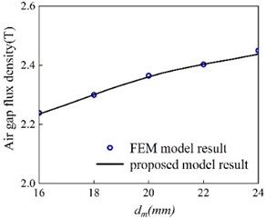
In no-load state, the MEC model that only changes the size of $d_{m}$ were calculated, and the corresponding finite element models were established for verification. As can be seen in Fig. 3, the results of the MEC model are reliable and can be used for subsequent braking force predictions.

Because the size of the air gap magnetic induction under no-load state is directly related to the size of the braking force, the no-load MEC model can already be used for the parameter design of ECB. By analyzing and calculating the model, the size parameters of PM and pole shoe can be obtained when the air-gap magnetic induction intensity and the permanent magnet utilization rate reach the maximum at the same time.

Fig. 3Air gap magnetic flux density varying with dm under no-load state

However, the generation of braking force also has a significant relationship with the secondary. The thickness and material of the inner conductor cylinder will affect the magnitude of the braking force, and the eddy current generated in the secondary will weaken the magnetic field strength generated by the primary. Therefore, in order to carry out the optimal design of ECB, it is necessary to obtain an analytical model that can predict the braking force.

2.2. Finite element model and braking force predict model of the EMB

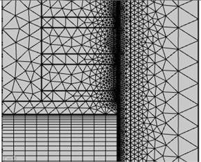
Finite element model have always been a popular method analyzing electromagnetic problems. FEM results can exhibit electromagnetic field distribution inside the structure and aid researchers analyze. In this section, axisymmetric 2-D FEM models of the ECB were performed, as shown in Fig. 4. The mesh size was taken very small at the air gap to get more accurate calculations.

Fig. 4Partial view of the finite element mesh model

The analytical model established in this paper only considers the ability of the ECB to generate braking force in a constant speed state, so the acceleration is set to 0 in the software. The parameterized calculation was set up with the speed being the parameter, and the parameter speed of 1-15 (m/s) were calculated for each model. The visualization results of the eddy current field intensity obtained by the finite element calculation are shown in Fig. 5, which shows patterns and variations of the distribution of electric fields.

It can be seen in Fig. 5 that the electric field intensity on the secondary section presents a relatively regular shape. And for different models, the deformation of electric field cross section shape with increasing velocity also have relatively consistent law.

Inspired by FEM visualization results, this paper attempts to calculate the eddy current and braking force of ECB using the mean value method by combining basic eddy current correlation formulae and electric field cross-section distribution. As shown in Fig. 6, the cross-section of electric field can be divided into three parts. Multiply the area of each part by the average value of electric field and add them together, the eddy current corresponding to one pole shoe can be calculate.

Fig. 5Cross-section diagram of electric field distribution at different velocities (Reproduced with permission from [Analytical modeling of permanent magnet linear eddy current brake using magnetic equivalent circuit method], IOS Press, 2022)

Cross-section diagram of electric field distribution at different velocities (Reproduced with permission from [Analytical modeling of permanent magnet linear eddy current brake using magnetic equivalent circuit method], IOS Press, 2022)

a) $v =$ 3 m/s

b) $v =$ 6 m/s

c) $v =$ 9 m/s

d) $v =$ 12 m/s

Fig. 6Schematic diagram of electric field section zoning

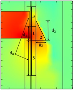
The division shown in Fig. 6 is based on the intensity, uniformity and distribution of electric field on the secondary. There are three parts obtained by the partition. The region 1 is the rectangular area in conductor cylinder with the highest electric field intensity. The region 2 is the triangle area with stronger electric field intensity in back iron. And the region 3 is the combination of two rectangle areas with the smaller electric field intensity in conductor cylinder. $d_{1}$ , $d_{2}$ , $d_{3}$ and $g_{2}$ are the side lengths of each area:

3

E = v \times B .

According to Eq. (3), the average value of the eddy current electric field intensity of each region, $E_{1}$ , $E_{2}$ and $E_{3}$ , can be obtained, as Eq. (4). $E_{1}$ is the mean value of electric field intensity in Region 1. For the electric field in this area is most concentrated, the magnetic flux density at the precise middle layer of conductor cylinder is taken for the calculation to obtain $E_{1}$ . For Region 2 where the electric field is relatively uniform. The mean electric field intensity $E_{2}$ is calculated using the magnetic flux density at the radius $(r_{0} + h_{b} / 4)$ in back iron. Region 3 is the area where electric field are gradually decreases above and below region 1, and areas of this two parts are small at top and large at bottom. The average electric field of the third region $E_{3}$ is calculated by $E_{1}$ times a velocity dependent coefficient $k_{E}$ :

4

\{\begin{array}{l} E_{1} = \frac{Φ_{δ}}{2 π d_{s} (r_{i} + \frac{h_{i}}{2})} v, \\ E_{2} = \frac{Φ_{δ}}{2 π d_{s} (r_{b} + \frac{h_{b}}{4})} v, \\ E_{3} = E_{1} k_{E} . \end{array}

The calculation of eddy current needs the mean values of electric field intensity of each region as well as their areas. And the side lengths of each region are relevant to both structure parameters and velocity, as follows:

5

\{\begin{array}{l} d_{1} = f (v, d_{s}, h_{i}), \\ g_{2} = g (v), \\ d_{3} = h (v, d_{s}, d_{m}, h_{i}) . \end{array}

Although if the coefficients could be directly multiplied by the structural parameters, as originally envisaged, the calculations could be simpler and clearer. However, through analyzing electric field results of different models, it is found that the side lengths are also sensitive to structural parameters: $d_{m}$ , $d_{s}$ , and $h_{i}$ .

To obtain the required side length, a series of finite element models were established. For each dimension parameter, three models were established, with other parameters remain unchanged, using the upper and lower bound of design range of that parameter and its intermediate value. The design range of parameters are given in Table 1. All the FEM models were calculated under the speed of 1–15 m/s.

Table 1Boundaries of design parameters

Parameter	$h_{p m}$ / mm	$h_{d}$ / mm	$h_{i}$ / mm	$d_{m}$ / mm	$d_{s}$ / mm
Upper bound	60	3	2	23	10
Lower bound	50	1	1	17	6

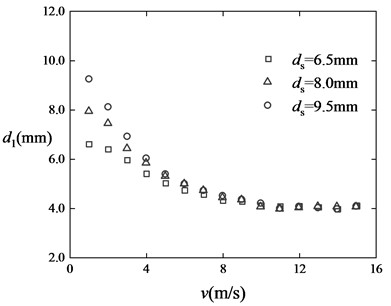
According to the correlation analysis of each edge length regarding ECB dimensional parameters, it is found that $d_{1}$ is mainly correlated with $v$ , $d_{s}$ , and $h_{i}$ , $g_{2}$ is mainly correlated with $v$ , $h_{i}$ , and $d_{3}$ is simultaneously correlated with $v$ , $d_{m}$ , $d_{s}$ , and $h_{i}$ . However, these correlations are simple and clear, as shown in Fig. 7, and direct formulae can be obtained by fitting the data. Only the correlation of a certain edge length with respect to velocity and one dimensional parameter is considered at a time, and a surface fit is performed using a custom function of the fitting tool. The custom function gives the main part of the function with speed as the main variable, plus the part of the function related to the size variable. The final fitted formulae for $d_{1}$ , $g_{2}$ , and $d_{3}$ are obtained as follows. Also, the formula of $k_{E}$ can be obtained by fitting.

Fig. 7Variation of d1 with velocity at different ds. Here, dsm, dmm, him are intermediate values of design range of ds, dm, hi

The values of the fitting results are given in Table 2 and the same in the following equations:

6

\begin{array}{l} d_{1} = A 3 v^{3} + A 2 v^{2} + A 1 v + A 0 + (d_{s} - d_{s m}) (A 21' v^{2} + A 11' v + A 01') \\ + (h_{i} - h_{i m}) (A 21^{'' v^{2}} + A 11^{''} v + A 01^{''}), \end{array}

7

g_{2} = B 2 v^{2} + B 1 v + B 0,

8

\begin{array}{l} d_{3} = C 3 v^{3} + C 2 v^{2} + C 1 v + C 0 + (d_{s} - d_{s m}) (C 31' v^{3} + C 21' v^{2} + C 11' v + C 01') \\ + (h_{i} - h_{i m}) (C 31'' v^{3} + C 21'' v^{2} + C 11'' v + C 01'') \\ + (d_{m} - d_{m m}) (C 21^{''' v^{2}} + C 11^{'''} v + C 01^{'''}), \end{array}

9

k_{E} = \{\begin{array}{l} D 21 v^{2} + D 11 v + D 01, (v \leq 3), \\ D 22 v^{2} + D 12 v + D 02, (v > 3) . \end{array}

Table 2The values of the fitting results

A3	−1.945×10⁻⁶	A2	8.414×10⁻⁵	A1	−0.001186	A0	0.009542
A2′	0.007877	A1′	−0.172	A’	0.8901
A2″	0.003325	A1″	0.05862	A″	−0.3998
B2	2.75×10⁻⁶	B1	−1.93×10⁻⁴	B0	0.00308
C3	1.641×10⁻⁶	C2	−9.39×10⁻⁵	C1	0.001521	C0	0.007323
C31′	0.002251	C21′	−0.06383	C11′	0.4854	C01′	−0.3865
C31″	0.004573	C21″	−0.1141	C11″	0.7963	C01″	0.4449
C21‴	0.001037	C11‴	0.009675	C01‴	0.2652
D21	0.02316	D11	−0.1646	D01	1.1172
D22	0.002624	D12	−0.0591	D02	1.041
K4	3.5×10⁻⁵	K3	−1.595×10⁻³	K2	0.02725	K1	−0.1742
K31′	0.01701	K21′	1.084	K11	−17.47	K01′	−37.61
K22′	−238.7	K12′	4212	K02′	−9285	K0	0.8173
K31″	−0.6055	K21″	21.52	K11″	−235.5	K01″	1114
K22″	−3746	K12″	7.54×10⁴	K02″	−4.451×10⁵

After obtaining the required parameters, the calculation of the vortex can be performed:

10

J_{1} = E_{1} σ_{i}, J_{2} = E_{2} σ_{b}, J_{3} = E_{3} σ_{i},

11

I = J_{1} \cdot d_{i} h_{i} + J_{2} \cdot \frac{1}{2} d_{2} g_{2} + J_{3} \cdot d_{3} h_{i},

where, $σ_{i}$ , $σ_{b}$ are conductivity of conductor cylinder and back iron, $J_{1}$ , $J_{2}$ , $J_{3}$ are average current density of three regions. With Eqs. (10-11), eddy current can be obtained by multiplying the current density by the cross section through which the current flows:

12

F_{i} = I \cdot k_{I} .

The Magneto Motive Force (MMF) $F_{i}$ generated by eddy current is given in Eq. (12). This is an approach similar to that used by the motor model, except that the MMF is not produced by coils, but by eddy current. The $F_{i}$ , an element represents the influence of eddy current in the MEC model, was calculated by multiplication of the eddy current in secondary and a coefficient relate to velocity ( $k_{I}$ ).

Different from motors, the eddy current induced in ECB is placed at the position in the secondary facing pole shoes instead of permanent magnets. Therefore, the coefficient $k_{I}$ was introduced, representing the influence of relative position of permanent magnet and eddy current in the MEC model. The relative position of permanent magnet and eddy current changes when the velocity changes, as shown in Fig. 8. As the electric field shift downward, the relationship between its induced magnetic field and the original field is more like overlap rather than intersection, which will cause the induced magnetic field to weaken the original field more seriously. Through analyzing FEM models built before, the coefficient $k_{I}$ under different condition was obtained.

Fig. 8Schematic diagram of induced magnetic field of eddy currents at different speeds (Reproduced with permission from [Analytical modeling of permanent magnet linear eddy current brake using magnetic equivalent circuit method], IOS Press, 2022)

Schematic diagram of induced magnetic field of eddy currents at different speeds (Reproduced with permission from [Analytical modeling of permanent magnet linear eddy current brake using magnetic equivalent circuit method], IOS Press, 2022)

a) At a lower velocity

b) At a higher velocity

Similarly, it can be obtained analytically that, in addition to velocity, $k_{I}$ also has a clear correlation with $d_{s}$ and $h_{i}$ . A polynomial of the fourth power of $x (v)$ and the second power of $y (d_{s} / h_{i})$ was obtained with an $R^{2}$ that higher than 0.99:

13

\begin{array}{l} k_{I} = K 4 v^{4} + K 3 v^{3} + K 2 v^{2} + K 1 v + K 0 \\ + (d_{s} - d_{s m}) (K 31' v^{3} + K 21' v^{2} + K 11' v + K 01' + K 22' v^{2} d_{s} + K 12' v d_{s} + K 02' d_{s}) \\ + (h_{i} - h_{i m}) (K 31^{'' v^{3}} + K 21^{'' v^{2}} + K 11^{''} v + K 01^{''} + K 22^{'' v^{2} h_{i}} + K 12^{''} v h_{i} + K 02^{'' h_{i}}), \end{array}

14

\{\begin{array}{l} P_{1} = \frac{J_{1}^{2}}{σ_{i}} π d_{1} (r_{o}^{2} - r_{i}^{2}), \\ P_{2} = \frac{J_{2}^{2}}{σ_{b}} (\frac{π d_{2}}{3} (r_{g}^{2} + r_{g} r_{o} + r_{o}^{2}) - π d_{2} r_{o}^{2}), \\ P_{3} = \frac{J_{3}^{2}}{σ_{i}} π d_{3} (r_{o}^{2} - r_{i}^{2}), \end{array}

15

F = \frac{n_{p s} (P_{1} + P_{2} + P_{3})}{v},

where $n_{p s}$ is the number of pole shoe, $r_{g} = r_{b} + g_{2}$ .

The braking force generated by eddy current was achieved by dividing the heat loss power of eddy current by speed.

To calculate the MEC model with relative velocity, iterative calculation was applied. Firstly, the radial flux density of the secondary was calculated under no-load condition, and eddy current was calculated accordingly. Then, the MEC model with MMF $F_{i}$ was recalculated, and iterative calculation was carried out. When the eddy current converges, the MEC model result was obtained, and the braking force can be gained accordingly. The complete calculation flow chart is shown in Fig. 9.

2.3. Prototype test

The ECB in this paper adopts a cylindrical structure, which is different with the commonly studied ECB. Therefore, its theoretical correctness and practical feasibility still need to be verified through prototype testing. An overall scaled-down prototype was used for impact tests. At the same time, the corresponding FEM model was established for verification.

In this study, the basic design goal of this ECB is to require a braking force greater than 120 kg while being reasonably sized. However, after preliminary design, the diameter and length of the prototype obtained are too large. Although its acceptable for the Practical mechanical application. The test equipment for it will need special design and manufacture. Therefore, a small prototype was made with its overall size being reduced to one third of the initial design. The main dimensions and material parameters of the prototype are demonstrated in Table 3. The PM type used to make the ECB is NdFeB, the material of cylinder conductor is aluminum alloy (6061). The shaft is made of stainless steel, the pole shoes and the back iron are made of ordinary carbon steel.

Fig. 9Calculation flow chart of ECB analysis model

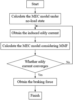
Table 3Dimensions and material parameters of the prototype

Parameter	Value	Parameter	Value
$r_{0}$	6 mm	$h_{a}$	0.5 mm
$r_{p m}$	17.5 mm	$h_{i}$	2 mm
$r_{i p}$	19.5 mm	$B_{r}$	1.25 T
$r_{e b}$	29 mm	$σ_{i}$	28 MS/m
$d_{m}$	10 mm	$σ_{b}$	6.9 MS/m
$d_{s}$	5 mm	$n_{p m}$	8
$n_{p s}$	9

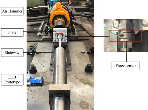
The experimental platform configuration is illustrated in Fig. 10. The outer cylinder of the ECB was fixed leaving a braking distance at the end, and the other side of the primary’s moving shaft was attached to an L-shaped plate with a slide rail underneath it. In order to obtain a higher relative speed of motion, an air hammer was used to impact onto the plate, causing the moving rod to carry the primary to move. The linear relative motion between the primary and the secondary was guaranteed by two guide rings placed beside pole shoes at both ends of the prototype. Therefore, the measured force value was the combination of braking force and friction force. To obtain the ECB brake force, the friction force should be subtracted, which comes from the mass of the prototype.

A FEM model with the parameters with the same parameters as the prototype was established. If the correctness of the finite element model can be found by testing, then the proposed model can be validated using the finite element model under other design parameters. Fig. 11 shows the braking force results obtained by experiment, proposed method, and FEM model. A good agreement between the three results can be observed. And it is visible that the braking force obtained by the proposed method is slightly greater than experimental results. This is because the pitch number of the prototype is too small, making the edge effect in the model to emerge. In addition, it should be mentioned that the design parameters of the prototype are actually smaller than the design range given above, but the obtained results are still accurate because the proportion of its structural dimensions does not change much.

Fig. 10Experimental platform configuration

It can be seen from Fig. 11 that the larger speed is difficult to realize by small prototype test. And in order to verify the proposed method with different design parameters, FEM models will be carried out in next chapter. In the following analysis, the pitch number will be set relatively large to minimize the edge effect. And the ECB is studied without considering temperature change, which are all assumed to be 20 °C.

The braking force of the ECB is nonlinear with respect to velocity, and although the prototype was tested at only 8 m/s, it already shows a nonlinear trend that matches the FEM results. This nonlinear nature is due to the fact that with increasing speed leads to enhanced eddy currents but the counter effect of the eddy currents on the primary electromagnetic field also increases (the region of high intensity of the eddy current electric field shrinks). As speed increases, the positive effect of speed on the eddy current electric field gradually outweighs the negative effect of the shrinking area of the high intensity region of the electric field on the eddy current, and thus the braking force characteristics are nonlinear. And the effect of design parameters on braking force characteristics is well worth analyzing.

3. Parametric analyze

3.1. Air gap

Using the ECB braking force prediction model proposed above, the influence of design parameters on the braking force results can be analyzed, which will guide the following optimal design of the ECB.

The width of the air gap is one of the most direct factors affecting the magnetic induction intensity of the air gap. Keep other parameters unchanged, FEM models are built with different air gap widths. FEM models and the proposed model are calculated to obtain the braking force results as shown in the Fig. 12. Comparing the finite element results, it can be seen that the prediction model proposed in this paper can predict the influence of the air gap width on the braking force.

It is obvious from the MEC model that the narrower the air gap, the smaller the air gap reluctance and the stronger the magnetic field in the air gap and in the secondary. However, for extremely narrow air gaps, the machining accuracy of the parts is limited, and the difficulty of the installation of the conductor layer barrel and the back iron barrel will increase. Therefore, in order to guarantee successful installation and structural stability during braking, the air gap width will be set directly to the minimum achievable in the following sections.

Fig. 11Breaking force results comparison

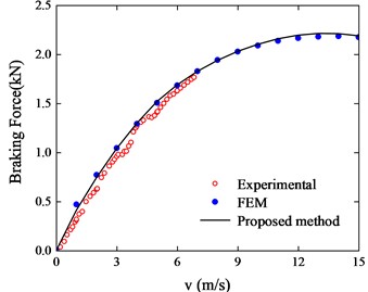
Fig. 12Braking force curve with different air gap widths

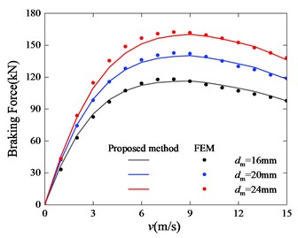
3.2. Permanent magnetic size parameters

The thickness and outer diameter of the permanent magnet ring determine the maximum magnetic energy that the ECB primary can deliver. Under the condition that other parameters remain unchanged, FEM models that only changes the thickness of the PM and FEM models that only changes the outer diameter of the PM are established. FEM models and the proposed model are calculated to obtain the braking force results as shown in the Figs. 13 14. It can be seen that the results of FEM and the proposed model both show that the magnitude of the braking force is positively related to the thickness and outer diameter of the permanent magnet. At the same time, the permanent magnet coefficients have little effect on the critical speed.

With other dimensions unchanged, the larger the permanent magnet ring, the stronger the magnetic field. However, the density of permanent magnets is relatively large (7.5 g/cm³), and the mass of the ECB also needs to be controlled and weighed in the design. In addition, if the outer diameter of the permanent magnet increases, it will lead to an increase in the diameter of the secondary, and eventually larger volume and mass of the ECB. And one of the optimization objective of the ECB design is, of course, smaller mass and volume.

Fig. 13Braking force curve with different outer diameter of the PM

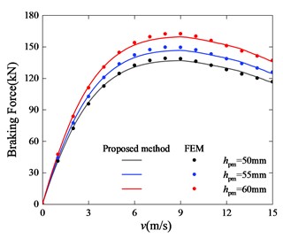
Fig. 14Braking force curve with different PM thickness

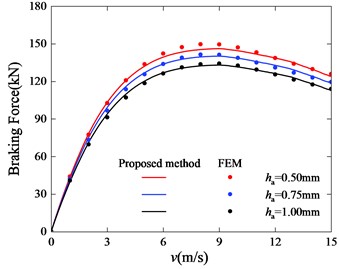
3.3. Pole shoe size parameters

According to the reluctance formula and the MEC model, the shape of the magnetic shoe affect the magnitude of the magnetic field generated by the primary. The thinner the pole shoe, the smaller the magnetic field intensity. At the same time, the magnetic saturation effect in pole shoes restrict the magnetic flux from increasing indefinitely.

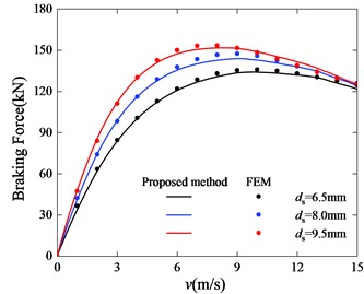
Under the condition that other parameters remain unchanged, FEM models that only changes the thickness of the PM and FEM models that only changes the outer diameter of the PM are established. FEM models and the proposed model are calculated to obtain the braking force results as shown in the Figs. 15, 16. It can be seen that the results of FEM and the proposed model both show that the size parameter of the magnetic shoe has a greater influence on the braking force when the speed is small. At the same time, the influence of the thickness of pole shoe on the critical speed is very obvious. When the thickness of the magnetic shoe increases from 6.5 mm to 9.5 mm, the critical speed is reduced from about 10 m/s to 7 m/s.

Fig. 15Braking force curve with different outer diameter of pole shoes

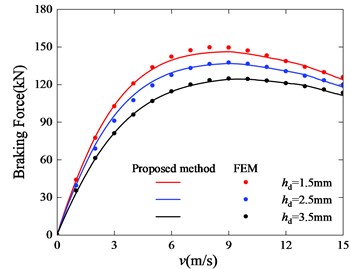
Fig. 16Braking force curve with different thickness of pole shoes

3.4. Cylindrical conductor

According to Eqs. (7-11), the thickness of the conductor cylinder directly affects the magnitude of eddy currents and braking force generated in the secondary. Under the condition that other parameters remain unchanged, FEM models and the proposed prediction model with different $h_{i}$ are established and calculated, and the braking force prediction results obtained are shown in the Fig. 17.

Fig. 17The braking force curve with different conductor cylinder thicknesses

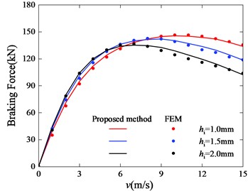
It can be seen from Fig. 17 that the critical speed decreases with the increase of $h_{i}$ . When the speed is greater than 6, the braking force attenuation caused by the increase of speed is aggravated with the growth of $h_{i}$ . The braking force curve of $h_{i}$ = 2 mm has no obvious advantage over the other two curves, and the critical speed is only about 6 m/s. Comparing the other two braking force curves, it can be seen that when the speed is less than 8 m/s, the braking force curve of $h_{i}$ = 1.5 mm is more advantageous, and when the speed is larger than 8 m/s, the braking force curve of $h_{i}$ = 1 mm is greater. But in choosing the optimal value of $h_{i}$ , its impact on critical speed needs more attention.

The braking force curve of different $h_{i}$ shows different trends, that is because the magnitude of the eddy current is obtained by multiplying the density of the eddy current by the cross-sectional area as Eq. (8). Since the magnetic permeability of the conductor is considered the same as that of air, the magnetic flux density and eddy current density in the conductor cylinder decrease significantly with the increase of its thickness. When the thickness exceeds a certain value, the gain of eddy current with the increase in the cross-sectional area will not be enough to offset the weakening of eddy current caused by the decrease of the eddy current density.

Based on the analysis in this chapter, it can be seen that the size parameters of the air gap and PMs can affect the braking force results as a whole without changing the braking force characteristics about the velocity. The parameters of the air gap are generally determined by mechanical design, while the parameters of PMs will affect the electromagnetic field of the ECB from the source, but too large PM volume will affect the mass of the ECB, so the parameters of the PM need to be optimized by gaming. Pole shoe related parameters are more likely to affect the braking force in the medium-speed phase of the performance, so its parameters should be optimized according to the specific operational requirements for the design. Conductor cylinder thicknesses have a greater impact on the braking force at high speeds and affect the volume and mass of the ECB, so this parameter needs to be optimized.

4. Multi-objective optimization problem and Stackelberg game theory

4.1. Multi-objective optimization problem

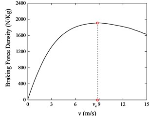
The design objective of ECB should be aligned with its application condition. For the special braking condition of strong impact load, the ECB should have its own consideration compared with existing researches. In the optimal design of the brake, it is always expected to obtain the maximum braking force, while keeping the overall weight under control. At the same time, the rated speed of the brake should be considered. The ECB designed in this paper is used to brake the movement of large impulse, so a large proportion will be in the state of high-speed movement during work. Therefore, the critical speed of the brake should be as large as possible.

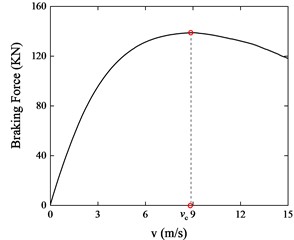
In the Fig. 18 is the braking force versus speed curve, braking force density is the braking force braking force divided by the mass of the ECB, and $v_{c}$ is the critical speed. In order to pursue the maximum braking force during the braking process, $F_{m v}$ is proposed as the optimization objective. The optimization model is established as follows:

16

F_{m v} = \sum_{v = 6}^{15} \frac{F}{M},

17

\{\begin{array}{l} m a x F_{m v} (X), v_{c} (X), \\ s . t . X \in Ω^{5} . \end{array}

The objective of this optimization problem is to maximize the ECB braking capability between certain parameter ranges and structural ratios, so there are no constraints other than the upper and lower regions of the variables. It is generally accepted that there is a scaling relationship limitation between $d_{m}$ and $d_{s}$ , but in the optimization, this scaling relationship in the optimal solution is always in accordance with the conventional limitation, so there is no need to give additional constraints. The range of variable selection is given by the upper and lower parameter limits below.

Multi-objective optimization methods have been widely used in the optimization design of mechanical structures. However, the traditional multi-objective optimization methods are often inefficient in solving the contradiction and containment between optimization objectives. Game theory is the mathematical theory and method of studying phenomena of a combat or competitive nature. It has been widely used in research in fields such as finance and political science. In recent years, some researches in mechanical design have integrated the game theory method into the multi-objective optimization algorithm, and achieved some results.

Fig. 18braking force and braking force density versus velocity

In the multi-objective optimization of ECB discussed in this paper, the two optimization objectives are somewhat conflicting. Generally speaking, the design objective of ECB hopes that the braking force is as high as possible, but while pursuing this optimization objective, the application conditions of ECB discussed in this paper need to pay attention to the braking force in the high-speed phase, i.e., it is hoped that the critical speed is as large as possible. The multi-objective optimization method applying game theory is suitable and more appropriate than the original method for the optimization problem in this paper.

Two game strategies have been introduced before, which are the Nash game strategy and the Stackelberg game strategy. In a Stackelberg game, there is a leadership relationship among the players. And in the ECB design problem discussed in this article, as optimization objectives, the braking force has a higher priority than the critical velocity. Therefore, the Stackelberg game strategy is suitable for the multi-objective optimization problem here.

4.2. Stackelberg game

A Stackelberg game consists of players, strategy and payoff. There are two types of player in Stackelberg game: one leader and one or multiple followers. Corresponding to the previous multi-objective optimization model, two players, leader and follower, were considered, and their objective functions are $F_{m v}$ and $v_{c}$ .

Table 4Range of design variables

Design variables	$x_{1}$ / mm	$x_{2}$ / mm	$x_{3}$ / mm	$x_{4}$ / mm	$x_{5}$ / mm
Upper bound	57.5	3.5	2	22	10
Lower bound	52.5	1.5	1	18	6

Table 5Material and parameters remaining constant

Parameter	Value	Parameter	Value
$r_{0}$	32 mm	$h_{a}$	0.5 mm
$h_{b}$	8 mm	$B_{r}$	1.45 T
$σ_{i}$	28 MS/m	$σ_{b}$	6.9 MS/m
$n_{p m}$	17	$n_{p s}$	18

The strategy is that the arrangement made by player be in response to the actions made by the other player. The strategy of leader and follower are made with corresponding sets of design variables: $x_{L}$ and $x_{F}$ . Before optimization, design variables in multi-objective optimization model need to be grouped in $x_{L}$ ( $x_{F}$ ), corresponding to two players.

According to the parametric analyze in the third chapter, the design variables ( $h_{p m}$ , $h_{d}$ , $h_{i}$ , $d_{m}$ , $d_{s}$ ) are set as $\{x_{1}, x_{2}, x_{3}, x_{4}, x_{5}\}$ . And they are grouped in $x_{L}$ $\{x_{1}, x_{2}, x_{3}\}$ and $x_{F}$ $\{x_{4}, x_{5}\}$ . The upper and lower bound of the design variables are given in Table 3. The value of other parameters of ECB are given in Table 4.

During the game, the leader first operates the optimizer to find min $(- F_{m v})$ by adjusting $x_{L}$ . Then, with $x_{L}$ remaining the result of leader, the follower operates the optimizer to find min ( $- v_{c}$ ) by adjusting $x_{F}$ . The $x_{F}$ is passed to the leaders move again and the two players take turns to find the optimization strategy. When the leader cannot improve its strategy, it is considered that a Stackelberg equilibrium is reached.

Algorithm 1 presents the workflow of this Stackelberg game model. Fmincon is used as the optimization solver for each player. And the number of iterations of the game is set to at least 8

The Stackelberg game has the characteristic that there can be two or multiple players with hierarchical relationship. In the Stackelberg game 1 given above, $(- F_{m v})$ was set as the leader player. According to its definition, min $(- F_{m v})$ simultaneously encapsulates the quest for greater braking force and less mass. With the characteristic of Stackelberg game, this Multi-objective optimization problem can also be transformed in a Stackelberg game with three players: $- F_{v}$ (leader), $- v_{c}$ (follower 1), Mass (follower 2). The calculation formula of $F_{v}$ is as Eq. (18). Mass is the total mass of the EBC calculated with design variables:

18

F_{v} = \sum_{v = 6}^{15} F .

Algorithm 1. Algorithmic procedure of the Stackelberg game 1.

Input: Initial design variables ( $x_{L}^{0}$ , $x_{F}^{0}$ ) and their upper and lower bounds of $x_{L}$ , $x_{F}$ .

(1) repeat

(2) Leader’s optimization: Taking ( $x_{L}^{0}$ , $x_{F}^{0}$ ) as initial design variables, keep $x_{F}^{0}$ as constant and adjust $x_{L}$ to minimize ( $- F_{m v}$ ) by the optimizer. Export new design variables ( $x_{L}^{n}$ , $x_{F}^{0}$ ).

(3) Follower’s optimization: Taking ( $x_{L}^{n}$ , $x_{F}^{0}$ ) as initial design variables, keep $x_{L}^{n}$ as constant and adjust $x_{F}^{0}$ to minimize (− $v_{c}$ ) by the optimizer. Export new design variables ( $x_{L}^{n}$ , $x_{F}^{n}$ ) and optimization results of the two player’s. Calculate the convergence index delta_x = abs( $F_{m v}$ ( $x_{L}^{n}$ , $x_{F}^{n}$ ) − $F_{m v}$ ( $x_{L}^{0}$ , $x_{F}^{0}$ ))

(4) ( $x_{L}^{0}$ , $x_{F}^{0}$ ) = ( $x_{L}^{n}$ , $x_{F}^{n}$ ).

(5) until the Stackelberg equilibrium is satisfied.

In game2, the design variables were regrouped in $x_{L}$ $\{x_{2}, x_{3}\}$ , $x_{F 1}$ $\{x_{4}, x_{5}\}$ and $x_{F 2}$ $\{x_{1}\}$ . The workflow of this Stackelberg game model 2 is given in Algorithm 2.

Algorithm 2. Algorithmic procedure of the Stackelberg game 2.

Input: Initial design variables ( $x_{L}^{0}$ , $x_{F 1}^{0}$ , $x_{F 2}^{0}$ ) and their upper and lower bounds of $x_{L}$ , $x_{F 1}$ , $x_{F 2}$ .

(1) repeat

(2) Leader’s optimization: Taking ( $x_{L}^{0}$ , $x_{F 1}^{0}$ , $x_{F 2}^{0}$ ) as initial design variables, keep $x_{F 1}^{0}$ , $x_{F 2}^{0}$ as constant and adjust $x_{L}$ to minimize (− $F_{v}$ ) by the optimizer. Export new design variables ( $x_{L}^{n}$ , $x_{F 1}^{0}$ , $x_{F 2}^{0}$ ).

(3) Follower1’s optimization: Taking ( $x_{L}^{n}$ , $x_{F 1}^{0}$ , $x_{F 2}^{0}$ ) as initial design variables, keep $x_{L}^{n}$ , $x_{F 2}^{0}$ as constant and adjust $x_{F 1}^{0}$ to minimize (− $v_{c}$ ) by the optimizer. Export new design variables ( $x_{L}^{n}$ , $x_{F 1}^{n}$ , $x_{F 2}^{0}$ ).

(4) Follower2’s optimization: Taking ( $x_{L}^{n}$ , $x_{F 1}^{n}$ , $x_{F 2}^{0}$ ) as initial design variables, keep $x_{L}^{n}$ , $x_{F 1}^{n}$ as constant and adjust $x_{F 2}^{0}$ to minimize (Mass) by the optimizer. Export new design variables ( $x_{L}^{n}$ , $x_{F 1}^{n}$ , $x_{F 2}^{n}$ ) and optimization results of the three player’s. Calculate the convergence index delta_x = abs( $F_{v}$ ( $x_{L}^{n}$ , $x_{F 1}^{n}$ , $x_{F 2}^{n}$ ) − $F_{v}$ ( $x_{L}^{0}$ , $x_{F 1}^{0}$ , $x_{F 2}^{0}$ )).

(5) ( $x_{L}^{0}$ , $x_{F 1}^{0}$ , $x_{F 2}^{0}$ ) = ( $x_{L}^{n}$ , $x_{F 1}^{n}$ , $x_{F 2}^{n}$ ).

(6) until the Stackelberg equilibrium is satisfied.

4.3. Game results and analysis

The convergence process of game 1 is shown in Fig. 19, which shows the decision result history of the two players $F_{m v}$ and $- v_{c}$ . As can be seen from the figure, the leader’s value has been greatly improved, while the follower’s value ( $- v_{c}$ ) has decreased slightly. The reason of the $v_{c}$ value does not increase is that it is difficult to increase the critical speed greatly due to the ECB structure and characteristic of the braking force versus speed curve. Generally, in this structure, increasing the braking force value will reduce the critical speed with a high probability. So it can be considered that the game result of the follower is still good.

Fig. 19Convergence histories of the two players of Stackelberg game 1

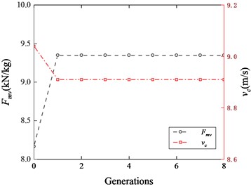
Fig. 20Convergence histories of players Fv and Mass of Stackelberg game 2

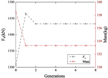
Fig. 20 shows the convergence history of the leader $F_{v}$ and follower2 Mass in game 2. The convergence history of $v_{c}$ is not given, because it is exactly the same as in game 1. It can be seen from the figure that $F_{v}$ achieves a higher numerical result in the first generation. However, reacting to the strategy of follower Mass, the numerical result of $F_{v}$ decreases in the next generation, and then quickly reaches equilibrium.

The equilibrium results of the two game models are shown in Table 6. It can be seen that the two results are exactly the same. Analyzing this result, it can be considered that $F_{m v}$ can be used as the optimization objective for the maximum braking force and minimum mass at the same time, and it is more concise in the Stackelberg game algorithm.

Game 2 shows the game process between braking force and mass, i.e., it can be better applied when targeting the contradiction between this two objectives and obtaining a braking force-dominated optimization result. Meanwhile, convergence was reached in one iteration in game 1. Although the convergence of the Stackelberg game is often reached quickly between 2 and 3 iterations when applied to multi-objective optimization related to mechanical design, it is still considered that after the grouping of variables the two optimization objectives does not have a major influence on each other. Due to the grouping of variables and the conservative selection of variables in this game design, it did not show too much contradiction between braking force and critical speed. Therefore, it is considered to try to present more design variables, such as the conductivity of the inner cylinder, and new grouping method in the subsequent optimization design. This game provides guidance for future optimized designs of ECBs under practical operating conditions.

Table 6Values of design variables

Variables	$x_{1}$ / mm	$x_{2}$ / mm	$x_{3}$ / mm	$x_{4}$ / mm	$x_{5}$ / mm
Original design	55.0	2.5	20	1.5	8.5
Stackelberg equilibrium for game 1	52.5	1.5	22	1.5	8.0
Stackelberg equilibrium for game 2	52.5	1.5	22	1.5	8.0

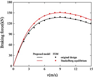
A FEM model is built using the equilibrium point data. Fig. 21 shows the braking force versus velocity curves of the ECB model at the initial design and equilibrium points, calculation results are obtained using the proposed model and FEM models. By comparing the data, it can be seen that the overall braking force has been improved, and the maximum braking force value has been increased from 1.37 kN in the initial design to 1.51 kN. In the meantime, the critical velocity did not decrease significantly, and according to the parameters in Table 6, it can be seen that the overall mass is reduced.

Fig. 21Braking force curve of original design and equilibrium point

Using the Stackelberg game strategy, the design parameters and design objectives were balanced after the game. Compared with the previous design, a more appropriate design and optimization model was obtained with better results on both sides of the design objectives. It shows that the Stackelberg game can better deal with this kind of problem where there are dominant optimization objectives and at the same time the conflict between the optimization objectives can be reconciled by the design parameters.

The above results indicate that the Stackelberg game strategy can be used in the multi-objective optimization of ECB, and the proposed model together with the Stackelberg game model can be applied in the optimal design of EBC.

5. Conclusions

Combined with the MEC model and a small amount of finite element analysis, this paper presents an analytical model that can approximately predict the braking force of ECB. In this model, the braking force is calculated through an approximate electric field cross section method. And the influence of eddy current on the MEC model is considered by introducing the MMF generated by eddy current. This analytical model is validated through small prototype experiments and finite element models. Although needs the reference of a small number of FEM models, this model can be reliable in a relatively large range.

The linear ECB structure studied in this paper has the design requirements of large braking force and fast working speed. After analyzing the design requirements and design parameters of ECB, a multi-objective optimization model is established using the Stackelberg game strategy. The optimization results are verified through FEM model calculation, and it is proved that the game method can be applied in the multi-objective optimization design of ECB.

The approximate calculation results obtained by the prediction model are not yet completely accurate. Therefore, this multi-objective optimization model is also only suitable for the preliminary parameter design of ECB. A more refined finite element model or model of Maxwell’s equations is also necessary. In addition, the existence of acceleration is certain in practical applications of ECB, and when the acceleration is large, it will also cause errors in the model. Therefore, taking into account acceleration and other factors to obtain a more accurate prediction model is a feasible direction for continued research. At the same time, the game method can also be considered to be applied to other ECB multi-objective optimization problems.

References

J. Tian, D. Li, and L. Ye, “Study on braking characteristics of a novel eddy current-hydraulic hybrid retarder for heavy-duty vehicles,” IEEE Transactions on Energy Conversion, Vol. 35, No. 3, pp. 1658–1666, Sep. 2020, https://doi.org/10.1109/tec.2020.2978304

Publisher
B. Ebrahimi, “Development of hybrid electromagnetic dampers for vehicle suspension systems,” University of Waterloo, Canada, 2009.

Search CrossRef
Wang et al., “Experimental study on vibration control of a model footbridge by a tiny ed-dy-current tuned mass damper with permanent magnets,” (in Chinese), Journal of Vibration and Shock, Vol. 33, No. 20, pp. 129–132, 2014, https://doi.org/10.13465/j.cnki.jvs.2014.20.025

Publisher
F. Sugai, S. Abiko, T. Tsujita, Xin Jiang, and M. Uchiyama, “Development of an eddy current brake system for detumbling malfunctioning satellites,” in IEEE/SICE International Symposium on System Integration (SII 2012), Dec. 2012, https://doi.org/10.1109/sii.2012.6427330

Publisher
D. Schieber, “Braking torque on rotating sheet in stationary magnetic field,” Proceedings of the Institution of Electrical Engineers, Vol. 121, No. 2, p. 117, Jan. 1974, https://doi.org/10.1049/piee.1974.0021

Publisher
D. Schieber, “Force on a moving conductor due to a magnetic pole array,” Proceedings of the Institution of Electrical Engineers, Vol. 120, No. 12, p. 1519, Jan. 1973, https://doi.org/10.1049/piee.1973.0311

Publisher
Seok-Myeong Jang, Sang-Sub Jeong, and Sang-Do Cha, “The application of linear Halbach array to eddy current rail brake system,” IEEE Transactions on Magnetics, Vol. 37, No. 4, pp. 2627–2629, Jul. 2001, https://doi.org/10.1109/20.951256

Publisher
J. Ge, X. Xie, Q. Sun, and G. Yang, “Design and dynamic characteristics of a double-layer permanent-magnet buffer under intensive impact load,” Journal of Sound and Vibration, Vol. 506, p. 116158, Aug. 2021, https://doi.org/10.1016/j.jsv.2021.116158

Publisher
Y. Jin, B. Kou, and L. Li, “Improved analytical modeling of an axial flux double-sided eddy-current brake with slotted conductor disk,” IEEE Transactions on Industrial Electronics, Vol. 69, No. 12, pp. 13277–13286, Dec. 2022, https://doi.org/10.1109/tie.2021.3139236

Publisher
B. Kou, W. Chen, and Y. Jin, “A novel cage-secondary permanent magnet linear eddy current brake with wide speed range and its analytical model,” IEEE Transactions on Industrial Electronics, Vol. 69, No. 7, pp. 7130–7139, Jul. 2022, https://doi.org/10.1109/tie.2021.3097603

Publisher
Kapjin Lee and Kyihwan Park, “Modeling eddy currents with boundary conditions by using Coulomb’s law and the method of images,” IEEE Transactions on Magnetics, Vol. 38, No. 2, pp. 1333–1340, Mar. 2002, https://doi.org/10.1109/20.996020

Publisher
B. Kou, Y. Jin, H. Zhang, L. Zhang, and H. Zhang, “Nonlinear analytical modeling of hybrid-excitation double-sided linear eddy-current brake,” IEEE Transactions on Magnetics, Vol. 51, No. 11, pp. 1–4, Nov. 2015, https://doi.org/10.1109/tmag.2015.2442583

Publisher
Wolfgang et al., “Modeling of a permanent magnet synchronous machine with internal magnets using magnetic equivalent circuits,” IEEE Transactions on Magnetics, Vol. 50, No. 6, pp. 1–14, Jun. 2014, https://doi.org/10.1109/tmag.2014.2299238

Publisher
T. Lubin, S. Mezani, and A. Rezzoug, “Exact analytical method for magnetic field computation in the air gap of cylindrical electrical machines considering slotting effects,” IEEE Transactions on Magnetics, Vol. 46, No. 4, pp. 1092–1099, Apr. 2010, https://doi.org/10.1109/tmag.2009.2036257

Publisher
L. Zuo, X. Chen, and S. Nayfeh, “Design and analysis of a new type of electromagnetic damper with increased energy density,” Journal of Vibration and Acoustics, Vol. 133, No. 4, Aug. 2011, https://doi.org/10.1115/1.4003407

Publisher
A. Antonio, N. Rezazadeh, A. Polverino, and S. Beneduce, “Numerical study of ultrasonic guided wave in composite reinforced panels with different stiffener shapes,” Macromolecular Symposia, Vol. 411, No. 1, Oct. 2023, https://doi.org/10.1002/masy.202300018

Publisher
D. Perfetto, C. Pezzella, V. Fierro, N. Rezazadeh, A. Polverino, and G. Lamanna, “FE modelling techniques for the simulation of guided waves in plates with variable thickness,” Procedia Structural Integrity, Vol. 52, pp. 418–423, Jan. 2024, https://doi.org/10.1016/j.prostr.2023.12.042

Publisher
D. P. Morisco, S. Kurz, H. Rapp, and A. Mockel, “A hybrid modeling approach for current diffusion in rectangular conductors,” IEEE Transactions on Magnetics, Vol. 55, No. 9, pp. 1–11, Sep. 2019, https://doi.org/10.1109/tmag.2019.2914006

Publisher
H. Y. Zhang, Z. Q. Chen, X. G. Hua, Z. W. Huang, and H. W. Niu, “Design and dynamic characterization of a large-scale eddy current damper with enhanced performance for vibration control,” Mechanical Systems and Signal Processing, Vol. 145, No. 3, p. 106879, Nov. 2020, https://doi.org/10.1016/j.ymssp.2020.106879

Publisher
Kou et al., “Analysis and design of hybrid excitation linear eddy current brake,” IEEE Transactions on Energy Conversion, Vol. 29, No. 2, pp. 496–506, Jun. 2014, https://doi.org/10.1109/tec.2014.2307164

Publisher
X. Zhao, “Study on electromagnetic properties and braking performance of permanent magnet type eddy current retarder,” (in Chinese), Nanjing Agricultural University, 2009.

Search CrossRef
B. Ebrahimi, M. B. Khamesee, and F. Golnaraghi, “Eddy current damper feasibility in automobile suspension: modeling, simulation and testing,” Smart Materials and Structures, Vol. 18, No. 1, p. 015017, Jan. 2009, https://doi.org/10.1088/0964-1726/18/1/015017

Publisher
M. Nemec, D. W. Zingg, and T. H. Pulliam, “Multipoint and multi-objective aerodynamic shape optimization,” AIAA Journal, Vol. 42, No. 6, pp. 1057–1065, Jun. 2004, https://doi.org/10.2514/1.10415

Publisher
T. W. Athan and P. Y. Papalambros, “A note on weighted criteria methods for compromise solutions in multi-objective optimization,” Engineering Optimization, Vol. 27, No. 2, pp. 155–176, Sep. 1996, https://doi.org/10.1080/03052159608941404

Publisher
D. Sasaki et al., “ECCOMAS Multiobjective aerodynamic optimization of supersonic wings using navier-stokes equations,” in Cd Rom Proceedings of Eccomas, 2000.

Search CrossRef
J. Nash, “Non-cooperative games,” Annals of Mathematics, Vol. 54, No. 2, pp. 286–295, 1951.

Publisher
Z. Zhan, “The research and application of multi-objective optimization design method based on game theory,” (in Chinese), Zhejiang University, 2013.

Search CrossRef
Z. Tang, J.-A. Désidéri, and J. Périaux, “Multicriterion aerodynamic shape design optimization and inverse problems using control theory and Nash games,” Journal of Optimization Theory and Applications, Vol. 135, No. 3, pp. 599–622, Nov. 2007, https://doi.org/10.1007/s10957-007-9255-4

Publisher
J. Leskinen and J. Périaux, “Distributed evolutionary optimization using Nash games and GPUs – Applications to CFD design problems,” Computers and Fluids, Vol. 80, pp. 190–201, Jul. 2013, https://doi.org/10.1016/j.compfluid.2012.03.017

Publisher
H. Von Stackelberg, The Theory of the Market Economy. New York: Oxford University Press, 1952.

Search CrossRef
C. Li, Y.-H. Chen, H. Zhao, and H. Sun, “Stackelberg game theory-based optimization of high-order robust control for fuzzy dynamical systems,” IEEE Transactions on Systems, Man, and Cybernetics: Systems, Vol. 52, No. 2, pp. 1254–1265, Feb. 2022, https://doi.org/10.1109/tsmc.2020.3018139

Publisher
H. Wang et al., “Waveform design of missile-borne radar and jammer based on Stackelberg model,” (in Chinese), Journal of Signal Processing, Vol. 36, No. 1, pp. 42–49, 2020.

Search CrossRef
Z. Tang, “Multi-objective optimization strategies using adjoint method and game theory in aerodynamics,” Acta Mechanica Sinica, Vol. 22, No. 4, pp. 307–314, Jun. 2006, https://doi.org/10.1007/s10409-006-0014-9

Publisher
J. F. Wang and J. Periaux, “Multi-point optimization using GAs and Nash/Stackelberg games for high lift multi-airfoil design in aerodynamics,” in 2001 Congress on Evolutionary Computation, Vol. 1, Jan. 2023, https://doi.org/10.1109/cec.2001.934440

Publisher
J. Wang et al., “Single/two-objective aerodynamic shape optimization by a Stackelberg/adjoint method,” Engineering Optimization, Vol. 52, No. 5, pp. 753–776, May 2020, https://doi.org/10.1080/0305215x.2019.1618287

Publisher
Y. Fan, G. Yang, J. Li, H. Zhang, and L. Wang, “Analytical modeling of permanent magnet linear eddy current brake using magnetic equivalent circuit method,” International Journal of Applied Electromagnetics and Mechanics, Vol. 69, No. 1, pp. 67–86, May 2022, https://doi.org/10.3233/jae-210190

Publisher

About this article

Received

09 March 2024

Accepted

18 June 2024

Published

31 July 2024

SUBJECTS

Mechanical vibrations and applications

DOI

https://doi.org/10.21595/jve.2024.24065

Keywords

analytical modeling

eddy current brake

magnetic equivalent circuit

multi-objective optimization

Acknowledgements

The authors have not disclosed any funding.

Data Availability

The datasets generated during and/or analyzed during the current study are available from the corresponding author on reasonable request.

Author Contributions

Yumeng Fan: conceptualization, methodology, writing-original draft preparation. Guolai Yang: resources, data curation. Quanzhao Sun: conceptualization.

Conflict of interest

The authors declare that they have no conflict of interest.

This is an open access article distributed under the Creative Commons Attribution License, which permits unrestricted use, distribution, and reproduction in any medium, provided the original work is properly cited.

Previous article in issue Previous Next article in issue Next

Research article

2020 02 15

Thermoelastic vibration analysis of disc brake based on multi-physical field coupling method

Sen Zhang, Jian Zhang

Research article

2019 10 19

Design and analysis of magnetic circuit of permanent magnet eddy current brake

Yumeng Fan, Guolai Yang

Research article

2019 10 19

Magneto-thermal coupling analysis of the permanent magnet eddy current brake under intensive impact load

Lei Li, Guo-Lai Yang, Zi-Xuan Li

Research article

2019 10 19

Electromagnetic buffering considering PM eddy current loss under intensive impact load

Zi-Xuan Li, Guo-Lai Yang, Lei Li

Y. Fan, G. Yang, and Q. Sun, “Analytical modeling of cylindrical eddy current brakes and multi-objective optimization based on game theory,” Journal of Vibroengineering, Vol. 26, No. 6, pp. 1263–1283, Jul. 2024, https://doi.org/10.21595/jve.2024.24065

Copy Extrica

Copied to clipboard!

TY  - JOUR
DO  - 10.21595/jve.2024.24065
UR  - https://doi.org/10.21595/jve.2024.24065
TI  - Analytical modeling of cylindrical eddy current brakes and multi-objective optimization based on game theory
T2  - Journal of Vibroengineering
AU  - Fan, Yumeng
AU  - Yang, Guolai
AU  - Sun, Quanzhao
PY  - 2024
DA  - 2024/07/31
PB  - Extrica
SP  - 1263-1283
VL  - 26
IS  - 6
SN  - 1392-8716
SN  - 2538-8460
ER  - 

Copy Ris

Copied to clipboard!

 @article{Fan_2024, title={Analytical modeling of cylindrical eddy current brakes and multi-objective optimization based on game theory}, ISSN={2538-8460}, url={https://doi.org/10.21595/jve.2024.24065}, DOI={10.21595/jve.2024.24065}, journal={Journal of Vibroengineering}, publisher={JVE International Ltd.}, author={Fan, Yumeng and Yang, Guolai and Sun, Quanzhao}, year={2024}, month=jul }

Copy Bibtex

Copied to clipboard!

[1]Y. Fan, G. Yang, and Q. Sun, “Analytical modeling of cylindrical eddy current brakes and multi-objective optimization based on game theory,” Journal of Vibroengineering, Jul. 2024, doi: 10.21595/jve.2024.24065.

Copy IEEE

Copied to clipboard!

Fan, Yumeng, Guolai Yang, and Quanzhao Sun. “Analytical Modeling of Cylindrical Eddy Current Brakes and Multi-Objective Optimization Based on Game Theory.” Journal of Vibroengineering, July 31, 2024. https://doi.org/10.21595/jve.2024.24065.

Copy Chicago

Copied to clipboard!

Analytical modeling of cylindrical eddy current brakes and multi-objective optimization based on game theory

Abstract

1. Introduction

2. The linear PM ECB analysis MODEL

2.1. The structure and MEC model of the ECB

2.2. Finite element model and braking force predict model of the EMB

2.3. Prototype test

3. Parametric analyze

3.1. Air gap

3.2. Permanent magnetic size parameters

3.3. Pole shoe size parameters

3.4. Cylindrical conductor

4. Multi-objective optimization problem and Stackelberg game theory

4.1. Multi-objective optimization problem

4.2. Stackelberg game

4.3. Game results and analysis

5. Conclusions

References

About this article

Related Articles