Abstract
This study investigates the impact of the trailing effect on the accuracy of crack detection under high-speed conditions. Finite element simulation analysis was used to explore the effects of the trailing effect on the magnetic field distribution on the rail surface and compare the signal intensity and sensitivity at different detection positions. The optimal detection position with higher signal intensity and sensitivity was identified, and a probe structure suitable for electromagnetic non-destructive testing at high speeds was proposed. Experimental results show that at a detection speed of 20.0 m/s, this probe structure effectively quantifies cracks deeper than 1.0 mm, with relative errors and standard deviations within 10 %.
1. Introduction
Rolling contact fatigue (RCF) crack on the top surface of rail is one of the main hidden dangers in the safety of high-speed railway. In order to solve this problem, many researchers have carried out related research work [1-5]. Among them, J. Wilson et al. [6] used eddy current pulse thermal imaging (ECPT) technology to detect RCF cracks on the rail surface. However, in order to ensure that the position of the crack is fully heated and avoid image blur, the detection speed is limited. Gao Yunlai et al. [7] combined magnetic line of force detection (MFL) with ECPT, and proposed a multi-physical electromagnetic and thermal imaging detection method, which can effectively detect the natural cracks on the top surface of the rail, and has high imaging resolution and sensitivity. Wu Yingchun et al. [8-9] studied the velocity effect in the electromagnetic thermal imaging detection of rail RCF cracks, and found that in the process of dynamic thermal imaging, the eddy current on the rail surface will produce a shadow effect, which will affect the distribution of temperature field, and then affect the imaging of cracks. Feng Jiefan et al. [10] studied the detection of rail RCF micro-cracks and hidden defects by eddy current pulse thermal imaging, analyzed the detection signals of cracks of different sizes in frequency domain and time domain, and enhanced the image features of cracks by normalized difference and other classical algorithms. In addition, many institutions, such as University of Electronic Science and Technology, Nanjing University of Aeronautics and Astronautics, China Academy of Railway Sciences, have jointly carried out the research and development of multi-physical rapid detection instruments for rail RCF cracks, and achieved fruitful results [11-12]. Literature [13-14] designed a rail surface adaptive bearing mechanism based on magnetic force line detection, and built a rail surface damage detection system, which was verified by hand trolley and rail inspection car. Gao Bin et al. [15] built the electromagnetic thermal imaging detection system, and tested it on the laboratory turntable and the actual rail, and then used the tensor decomposition algorithm to process the detection signal under the velocity effect, which can effectively identify the crack characteristics. These researches provide some technical support for the detection of rail RCF cracks and have certain significance for ensuring the safety of high-speed railway.
Although some progress has been made in the quantitative detection of RCF cracks in high-speed rail, the realization of rapid on-line quantitative nondestructive testing of RCF cracks in high-speed rail still needs to be further studied. At present, some detection technologies are limited by the method and principle of detection speed, so they cannot achieve fast on-line inspection. At the same time, in the rapid non-destructive testing of high-speed rail, due to the improvement of testing speed, the speed effect will have an impact on the quantitative identification of RCF damage, and may lead to missed detection and misdetection of cracks. In order to ensure the safe operation of high-speed railway, it is very necessary to use non-destructive testing (NDT) technology to detect RCF damage, railway failure and health status of in-service rail.
Therefore, based on the DC electromagnetic nondestructive testing technology, the influence of the shadow effect on the magnetic field distribution on the rail surface is analyzed by finite element simulation. Aiming at the magnetic field distribution as a reference, we aim to optimize the detection signal strength and sensitivity, propose the optimal probe structure for fast moving conditions, and apply it to the rapid quantitative detection of rail RCF cracks. This research result provides an important basis for the development of probe structure with high sensitivity and high signal strength to realize the rapid and quantitative detection of rail cracks.
2. Simulation research on the optimal detection position
2.1. Establishment of finite element simulation model
When there is a relatively fast motion between the probe and the specimen, the distribution of the moving eddy current and magnetic field in the specimen will change due to the existence of the drag effect, which is significantly different from that of the magnetic field and eddy current in the static state. at this time, the best detection position is also changed. In order to study the best detection position in the state of fast motion, the finite element model is established according to the modeling method of reference [16], as shown in Fig. 1. The thickness of the rail specimen is set to 14.0 mm. In order to find the best detection position, 12 detection points are arranged under the excitation coil, in which the detection point is the location of the magnetic sensor in the traditional eddy current testing. In the simulation, the magnetic induction intensity axis component and magnetic induction intensity axis component at the detection point - are obtained respectively to carry out research. In addition, in order to study the distribution of the magnetic field on the surface of the specimen under the probe, a straight line is drawn on the surface of the specimen below the excitation coil, and the comprehensive magnetic induction intensity on the line is extracted. The lift-off setting is 1.0 mm and the DC excitation is 0.1 A. The physical and geometric parameters of the specimen and the excitation coil are shown in Tables 1-2.
Fig. 1Finite element simulation diagram
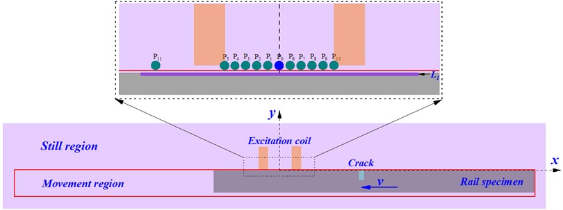
Table 1physical and geometric parameters of the excitation coil
Materials | Inner diameter | Outside diameter | Height | Number of turns | Electric conductivity | Relative permeability |
Copper | 10.0 mm | 15.0 mm | 8.0 mm | 500 | 58.0 MS/m | 1 |
Table 2Physical and geometric parameters of the specimen
Materials | Length | Thickness | Electric conductivity | Magnetic permeability |
1008 section steel | 250.0 mm | 8.0 mm | 2.0 MS/m | 1000 |
2.2. The influence of shadow effect on the quantitative detection of cracks
According to the simulation model in Fig. 1, this chapter first studies the influence of shadow effect on the quantitative characterization of cracks in DC electromagnetic nondestructive testing. When there is no crack on the surface of the specimen, the magnetic induction intensity on is obtained, and the relative position curve between and the excitation coil is drawn, as shown in Fig. 2.
Fig. 2Relative position curve of B0 and excitation coil at different speeds
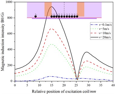
It can be seen from Fig. 2 that at low speed (0.1 m/s), the value of is small, and the moving eddy current is close to zero. With the increase of speed, the value increases significantly, and the magnetic field distribution on the specimen surface changes due to the influence of the shadow effect: the value increases gradually from right to left inside the excitation coil and reaches the maximum at the left edge of the excitation coil (below ); the minimum value of appears at the right edge of the excitation coil (below ); on the outside of the excitation coil, the value decreases as it moves away from the excitation coil. In addition, when the speed is more than 5.0 m/s, the value behind the phase motion of the excitation coil (left) is much larger than that of the front (right) of the excitation coil.
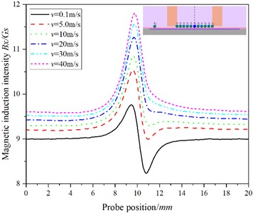
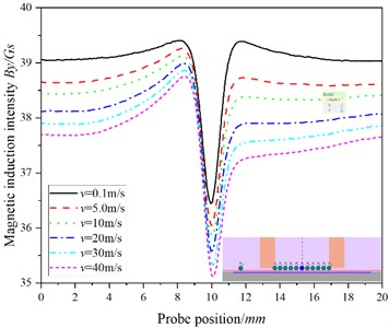
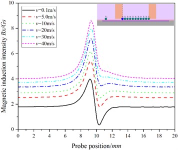
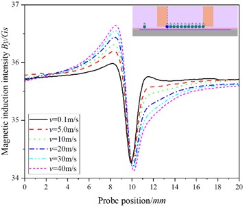
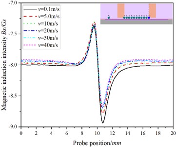
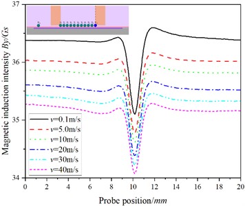
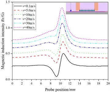
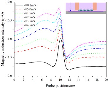
According to the magnetic field distribution on the surface of the specimen without crack obtained in Fig. 2, the influence of drag effect on quantitative electromagnetic nondestructive testing of crack is studied. When there are cracks on the surface of the specimen, the and by values at different positions and speeds are extracted for study, as shown in Figs. 3-6. Among them, is the traditional eddy current testing position; and correspond to the detection positions of the maximum and minimum magnetic induction intensity in the specimen, respectively; and is the detection position behind the movement of the excitation coil, which is used to study the shadow effect. The width of the crack is 0.8 mm and the depth is 2.0 mm.
Comparing Figs. 3-6, we can see that with the increase of speed, the baseline value of increases gradually, while that of decreases gradually. However, due to the existence of the shadow effect, the magnetic field distribution on the specimen surface changes, resulting in differences in the baseline values of magnetic induction intensity at different detection locations, and the change trends of and values obtained at different detection sites are obviously different: in Figs. 3 4 6, the values of and increase with the increase of speed.
Fig. 3The relationship between the position of the probe and the magnetic induction intensity at P0
a)
b)
Fig. 4The relationship between the position of the probe and the magnetic induction intensity at P5
a)
b)
Fig. 5The relationship between the position of the probe and the magnetic induction intensity at P10
a)
b)
In Fig. 5, with the increase of speed, the value of hardly changes, but the value of decreases gradually, which is obviously different from that of , and . Combined with Fig. 2, we can see that with the increase of speed, the shadow effect is more obvious, the maximum magnetic induction intensity in the specimen appears below the point, while the magnetic induction intensity at the is the smallest, and with the increase of the testing speed, the dynamic eddy current is more concentrated on the surface of the specimen, that is, the skin effect is more obvious, resulting in poor characterization of cracks at .
Fig. 6The relationship between the position of the probe and the magnetic induction intensity at P11
a)
b)
3. Selection of the best detection position under the condition of fast motion
3.1. Crack detection signals of different depths at each detection point
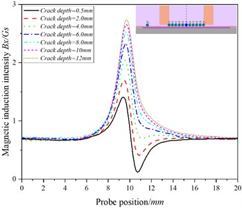
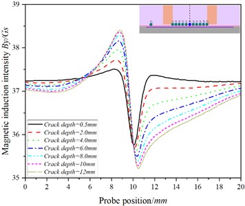
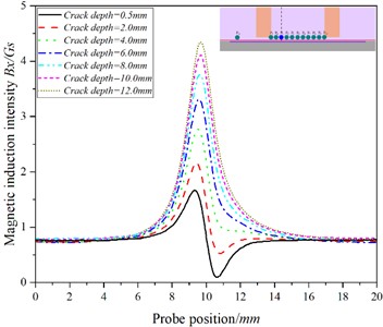
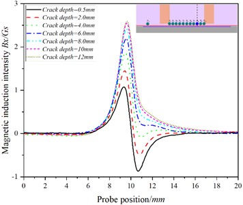
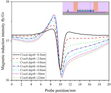
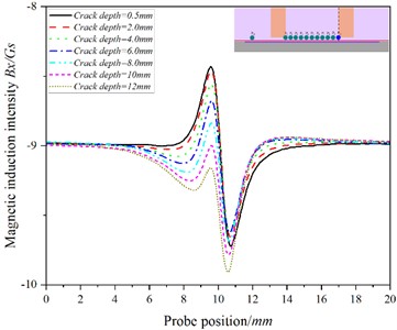
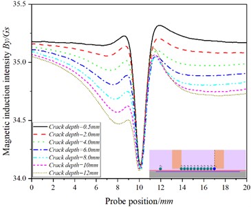
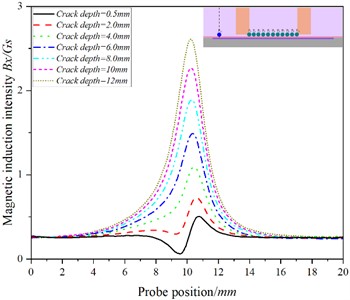
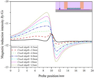
In order to study the relationship between crack depth and magnetic induction intensity at each detection point, the detection signals are selected when the detection speed is 20.00 m/s, crack width is 0.8 mm and depth is 0.5 mm-12.0 mm. The relationship curves between , and probe position at different depths from to are obtained respectively. Figs. 7-12 shows the curves of , and crack depth at different crack depths at , , , , and , respectively. The crack center corresponds to the axis 10.0 mm.
Fig. 7The curve of the relationship between the position of the probe and the magnetic induction intensity at the P0 when the detection speed is 20.00 m/s
a)
b)
It can be seen from Figs. 7(a)-12(a) that there are significant differences in the variation trend of detection signals with crack depth at different detection points: in Figs. 7(a)-9(a), the baseline value of increases in turn and reaches the maximum value at , while in Figs. 10(a)-11(a), the baseline value of gradually decreases to a negative value.
Fig. 8The curve of the relationship between the position of the probe and the magnetic induction intensity at the P3 when the detection speed is 20.00 m/s
a)
b)
Fig. 9The curve of the relationship between the position of the probe and the magnetic induction intensity at the P5 when the detection speed is 20.00 m/s
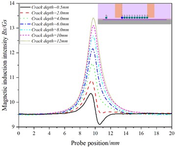
a)
b)
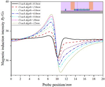
Fig. 10The curve of the relationship between the position of the probe and the magnetic induction intensity at the P8 when the detection speed is 20.00 m/s
a)
b)
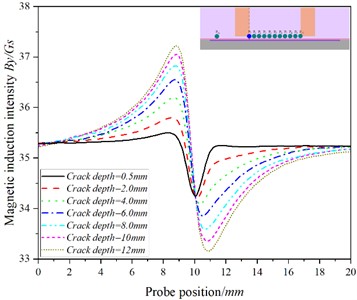
There is an abrupt change in at the crack, and the at - increases with the increase of crack depth, while at -, with the increase of crack depth, the increasing trend of gradually slows down, even showing that increases at first and then decreases with the increase of crack depth (as shown in Fig. 10(a) and Fig. 1(a)). The change trend of is consistent with that of - Figs. 7(b)-12(b) shows that in Fig. 7(b)-9(b), the baseline value of increases at first and then decreases, while in Figs. 10(b)-11(b), the baseline value of decreases in turn; at the crack, changes sharply, and By at - increases with the increase of crack depth. At -, with the increase of crack depth, gradually slows down with the crack depth, while at , decreases with the increase of crack depth. The at also increases with the depth of the crack.
Fig. 11The curve of the relationship between the position of the probe and the magnetic induction intensity at the P10 when the detection speed is 20.00 m/s
a)
b)
Fig. 12The curve of the relationship between the position of the probe and the magnetic induction intensity at the P11 when the detection speed is 20.00 m/s
a)
b)
3.2. Determination of the best detection location
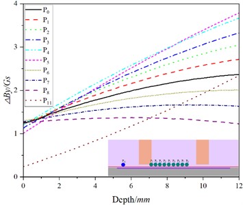
In order to obtain the best detection position, the and values of crack detection signals at different depths at each detection point are extracted, and the and values are fitted with the crack depth, as shown in Fig. 3. Because of the poor fitting relationship between the and values at and points and the crack depth, it is not shown in Fig. 13. In Fig. 13, the ordinate represents the strength of the detection signal, and the rate of change of the fitting curve with depth represents the sensitivity of the detection signal, and the greater the rate of change, the higher the sensitivity of the detection signal. It can be seen in Fig. 13 that there is a good quadratic function relationship between the values of and at each detection point and the crack depth, and the linear correlation coefficients are all above 0.99.
Fig. 13Fitting curve of difference peak value and crack depth at each detection point
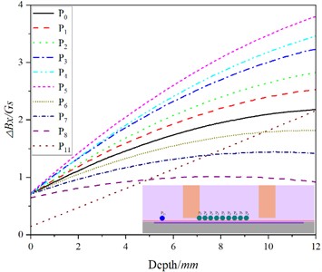
a)
b)
In Fig. 13(a), the detection sensitivity and signal intensity of each detection point are arranged from low to high as follows: , that is, affected by the shadow effect, the detection sensitivity and signal strength of the detection point on the left side of are increased in turn, while at the detection point on the right side of , the detection sensitivity and signal strength are weakened in turn. The detection signal strength and sensitivity are the highest at point. The detection sensitivity of position is between and , but because the position is far away from the excitation coil, the detection signal strength is lower than that of and .
The order of detection sensitivity from low to high in Fig. 13(b) is as follows: , which is the same as that in Fig. 13(a). The detection sensitivity and signal strength of position are the same as those described in Fig. 13(a). Considering the strength and sensitivity of the detection signal, the point can be determined as the best detection position.
4. Analysis and discussion of experimental results
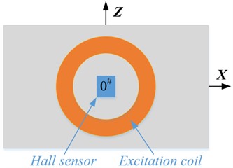
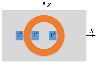
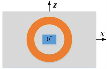
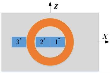
In order to verify the simulation results, the structure of the probe designed in this paper is shown in Fig. 14. In this experiment, eight Hall sensors numbered 0#, 1#, 2# and 3# are used to convert the magnetic induction intensity signal in the axis direction into the voltage signal output, and the Hall sensors numbered 0*, 1*, 2* and 3* are used to convert the magnetic induction intensity signal in the axis direction into the voltage signal output. Among them, probe 1 and probe 3 are traditional probe structures. In the simulation, the magnetic sensor is replaced by the detection point, but in practice, the volume of the magnetic sensor needs to be taken into account. Therefore, when designing probe 2 and probe 4, the Hall sensor 2#and 2* are as close to the edge of the excitation coil as possible (that is ). It should be pointed out that during the rotation of the turntable, the order in which the cracks pass through the Hall sensors in probe 2 (or probe 4) is 0#, 1#, 2# and 3# (or 0*, 1*, 2* and 3*).
In order to further determine the best detection position, According to the previous analysis, it can be seen that placing the Hall sensor at point is the best detection position.The gap between the Hall sensor and the excitation coil and track surface is 1 mm. each Hall sensor is arranged according to its placement position in Fig. 14, and the change trend of and output of each Hall sensor at different speeds is plotted, as shown in Fig. 15. In the Figure, the Abscissa shows the placement position of each Hall sensor near the probe; the ordinate reflects the and values of different depth cracks obtained by each Hall sensor, the ordinate value indicates the strength of the detection signal, and the different ordinate values corresponding to the same Abscissa value reflect the resolution of the Hall sensor to the crack depth.
Fig. 14Schematic diagram of probe structure
a) Probe 1
b) Probe 2
c) Probe 3
d) Probe 4
Fig. 15Output values of Hall sensors at different speeds
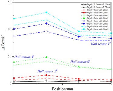
a)
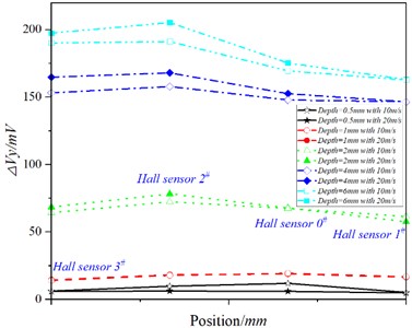
b)
As can be seen from Fig.15 (a), with the increase of speed, the position of at 0#, 1# and 3# increases slightly at the position of the Hall sensor, while the position of the Hall sensor increases significantly at the Hall sensor position. In addition, does not increase uniformly at all detection positions with the increase of velocity, but increases significantly in the opposite direction of the probe movement direction (near the position), that is, the shadow effect appears. In Fig. 15(b), when the crack depth is 0.5 mm and 1.0 mm respectively, the difference of the value of each Hall sensor is small; when the crack depth is 2.0 mm, 4.0 mm and 6.0 mm, it is obvious that the value of the 1# Hall sensor increases significantly with the increase of velocity, and the value of the 0# and 3# Hall sensor increases slightly. However, at the position of the 1# Hall sensor, except for the crack with a depth of 0.5 mm, the value decreases with the increase of . This is due to the fact that with the increase of velocity, the drag effect becomes more and more obvious, and the magnetic field moves in the opposite direction to the probe, so that the value of the position of the 1#Hall sensor decreases.
According to the above research, when there is a rapid relative motion between the probe and the specimen, the optimal probe structure is shown in Fig. 16, in which probe 5 is used to detect and probe 6 is used to detect . Fig. 16(a) shows that the probe moves at a certain speed and the specimen is still; Fig. 16(b) shows that the specimen moves at a certain speed and the probe is at rest, which is suitable for crack detection of fast-moving metal components.
Fig. 16Schematic diagram of the best probe structure
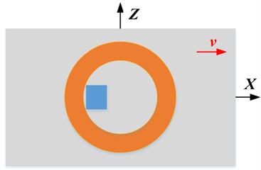
a) Probe moves, sample
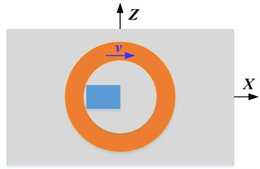
b) Probe still, sample moves
Fig. 17 shows the fitting curves of crack depth and detection signal at different speeds. It can be seen from Fig. 17(a) that there is a quadratic function relationship between crack depth and (), and the correlation coefficients are 0.994 and 0.996 respectively. Comparing the two curves in Fig. 17(a), it can be seen that is more sensitive to the change of crack depth. Fig. 17(b) shows the same trend, with a correlation coefficient of 0.996 for both curves. In addition, Fig.17 shows that the sensitivity of () to crack depth is higher at 20.0 m/s than that at 10.0 m/s.
Fig. 17Fitting curve of detection signal and crack depth at different speeds
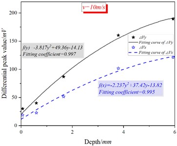
a) = 10 m/s
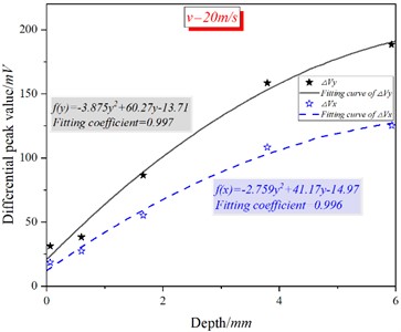
b) = 20 m/s
The fitting formula in Fig. 17 is inverted in order to realize the quantitative characterization of cracks in engineering practice, as shown in Table 3. In the table, and are the standard crack depth and the measured crack depth respectively, and is the relative error between the standard crack depth and the measured crack depth.
As can be seen from Table 3, except for cracks with a depth of 0.5 mm and 1.0 mm (blackbody thickening), the relative errors of other crack depths are all less than 10 %.The main reason for the higher relative error of the crack depth of 0.5 mm and 1.0 mm is that the signal strength of the shallow crack detection is lower, and it is more easily affected by vibration lift and noise signals, especially the crack with the depth of 0.5 mm. Compared with the inversion results in literature [17], the inversion accuracy of crack depth at the best detection location is greatly improved, especially when is used to invert the crack depth, it is further proved that the probe has better detection ability at the best detection location. At the same time, compared with the static PEC detection of literature [18], the probe structure can detect deeper RCF cracks under the condition of fast motion.
Table 3Inversion results of crack depth
= 10 m/s | = 20 m/s | |||||
(mm) | (mm) | (%) | (mm) | (mm) | (%) | |
(mV) | 0.5 | 0.65 | 30 | 0.5 | 0.61 | 22 |
1.0 | 0.83 | 17 | 1.0 | 0.88 | 12 | |
2.0 | 1.88 | 6 | 2.0 | 1.92 | 4 | |
4.0 | 4.16 | 4 | 4.0 | 4.27 | 6.75 | |
6.0 | 5.93 | 1.17 | 6.0 | 5.84 | 2.67 | |
(mV) | 0.5 | 0.62 | 24 | 0.5 | 0.63 | 26 |
1.0 | 0.87 | 13 | 1.0 | 0.84 | 16 | |
2.0 | 1.86 | 7 | 2.0 | 1.90 | 5 | |
4.0 | 4.25 | 6.25 | 4.0 | 4.16 | 4 | |
6.0 | 5.84 | 2.67 | 6.0 | 5.89 | 1.83 | |
5. Conclusions
This study examined the impact of the trailing effect on the magnetic field distribution and detection signals within the rail, identifying the optimal detection position for magnetic sensors in high-speed conditions. Based on these findings, we proposed an electromagnetic non-destructive testing probe structure suitable for detecting RCF cracks in rails. Experimental results show that at a detection speed of 20.0 m/s, the probe can effectively quantify crack depth when the crack depth is greater than 1.0 mm, with both relative error and standard deviation within 10 %.
References
-
V. Ramanan, A. Ramankutty, S. Sreedeep, and S. R. Chakravarthy, “Dynamical states of thermo-acoustic system with respect to frequency-phase relationship based on probabilistic oscillator model,” Nonlinear Dynamics, Vol. 110, No. 2, pp. 1633–1649, Jul. 2022, https://doi.org/10.1007/s11071-022-07693-z
-
X. Zhang, T. Sun, Y. Wang, K. Wang, and Y. Shen, “A parameter optimized variational mode decomposition method for rail crack detection based on acoustic emission technique,” Nondestructive Testing and Evaluation, Vol. 36, No. 4, pp. 1–29, Jul. 2020, https://doi.org/10.1080/10589759.2020.1785447
-
Y. Jiang, H. Gao, Q. Zhang, S. Zhang, X. Li, and Z. Li, “Evaluation of fatigue cracks on rail material based on laser nonlinear wave modulation and adaptive particle swarm optimization – support vector machines,” Nondestructive Testing and Evaluation, Vol. 38, No. 5, pp. 713–731, Sep. 2023, https://doi.org/10.1080/10589759.2022.2159961
-
J. Shen, L. Zhou, H. Rowshandel, G. L. Nicholson, and C. L. Davis, “Prediction of RCF clustered cracks dimensions using an ACFM sensor and influence of crack length and vertical angle,” Nondestructive Testing and Evaluation, Vol. 35, No. 1, pp. 1–18, Jan. 2020, https://doi.org/10.1080/10589759.2019.1611817
-
J. Zhang, P. Yu, and T. Gang, “Measurement of the ultrasonic scattering matrices of near-surface defects using ultrasonic arrays,” Nondestructive Testing and Evaluation, Vol. 31, No. 4, pp. 303–318, Oct. 2015, https://doi.org/10.1080/10589759.2015.1093626
-
J. Wilson, G. Tian, I. Mukriz, and D. Almond, “PEC thermography for imaging multiple cracks from rolling contact fatigue,” NDT and E International, Vol. 44, No. 6, pp. 505–512, Oct. 2011, https://doi.org/10.1016/j.ndteint.2011.05.004
-
Y. Gao, G. Y. Tian, K. Li, J. Ji, P. Wang, and H. Wang, “Multiple cracks detection and visualization using magnetic flux leakage and eddy current pulsed thermography,” Sensors and Actuators A: Physical, Vol. 234, pp. 269–281, Oct. 2015, https://doi.org/10.1016/j.sna.2015.09.011
-
H. Li et al., “Multiphysics structured eddy current and thermography defects diagnostics system in moving mode,” IEEE Transactions on Industrial Informatics, Vol. 17, No. 4, pp. 2566–2578, Apr. 2021, https://doi.org/10.1109/tii.2020.2997836
-
Y. Wu et al., “Induction thermography for rail nondestructive testing under speed effect,” in 2018 IEEE Far East NDT New Technology and Application Forum (FENDT), pp. 158–159, Jul. 2018, https://doi.org/10.1109/fendt.2018.8681985
-
L.-F. Feng, J.-P. Peng, K. Zhang, J. Bai, and X.-R. Gao, “Research on eddy current pulsed thermography for Squats in railway,” in Quantitative InfraRed Thermography, pp. 586–593, Jan. 2018, https://doi.org/10.21611/qirt.2018.062
-
X. Niu, J. Zhang, A. Croxford, and B. Drinkwater, “Efficient finite element modelling of guided wave scattering from a defect in three dimensions,” Nondestructive Testing and Evaluation, Vol. 38, No. 5, pp. 732–752, Sep. 2023, https://doi.org/10.1080/10589759.2022.2162050
-
G. Zhao, M. Jiang, Y. Luo, W. Li, and Q. Sui, “Comparison of sensitivity in nonlinear ultrasonic detection based on Lamb wave phase velocity matching mode,” Nondestructive Testing and Evaluation, Vol. 38, No. 2, pp. 297–312, Mar. 2023, https://doi.org/10.1080/10589759.2022.2121394
-
P. Wang, Y. Gao, G. Tian, and H. Wang, “Velocity effect analysis of dynamic magnetization in high speed magnetic flux leakage inspection,” NDT and E International, Vol. 64, pp. 7–12, Jun. 2014, https://doi.org/10.1016/j.ndteint.2014.02.001
-
Y. Bin, H. Chaojie, X. Fuzhen, L. Chengqiang, X. Yanxun, and X. Biao, “Health monitoring of pressure vessels based on ultrasonic guided waves i: wave propagation behavior and damage localization,” Journal of Mechanical Engineering, Vol. 56, No. 4, pp. 1–10, 2020.
-
B. Gao, P. Lu, W. L. Woo, G. Y. Tian, Y. Zhu, and M. Johnston, “Variational Bayesian subgroup adaptive sparse component extraction for diagnostic imaging system,” IEEE Transactions on Industrial Electronics, Vol. 65, No. 10, pp. 8142–8152, Oct. 2018, https://doi.org/10.1109/tie.2018.2801809
-
F. Yuan, Y. Yu, W. Wang, and G. Tian, “A novel probe of DC electromagnetic NDT based on drag effect: design and application in crack characterization of high-speed moving ferromagnetic material,” IEEE Transactions on Instrumentation and Measurement, Vol. 70, pp. 1–10, Jan. 2021, https://doi.org/10.1109/tim.2021.3069036
-
F. Yuan, Y. Yu, L. Li, and G. Tian, “Investigation of DC electromagnetic-based motion induced eddy current on NDT for crack detection,” IEEE Sensors Journal, Vol. 21, No. 6, pp. 7449–7457, Mar. 2021, https://doi.org/10.1109/jsen.2021.3049551
-
Z. Wang, Y. Fei, P. Ye, F. Qiu, G. Tian, and W. L. Woo, “Crack characterization in ferromagnetic steels by pulsed eddy current technique based on GA-BP neural network model,” Journal of Magnetism and Magnetic Materials, Vol. 500, p. 166412, Apr. 2020, https://doi.org/10.1016/j.jmmm.2020.166412
About this article

This work is supported by Natural Science Foundation of Guangdong Province (No. 2022A1515011409); supported by Key Areas Special Project of General Universities in Guangdong Province (No. 2023ZDZX1024);supported in part by research grants from the Youth Project of National Natural Science Foundation of China (No. 52105268); supported in part by the Key Project of Shaoguan University (No. SZ2017KJ08; SZ2020KJ02; 2024KJ06); supported in part by the Natural Science Foundation of Guangdong Province under Grant 2023A1515011253, in part by the Natural Science Foundation of Chongqing under Grant CSTB2022NSCQMSX1386, in part by the Higher education institution featured innovation project of Department of Education of Guangdong Province under Grant 2023KTSCX138, in part by the Science and Technology Project of Shaoguan City under Grant 230330098033679,in part by Shaoguan University Ph.D. Initiation Project (No. 440-9900064602).supported in part by Shaoguan University Ph.D. Initiation Project (440-9900064604); supported by Shao guan Social Development Science and Technology Collaborative Innovation System Construction Project (No. 230330178036242).
The datasets generated during and/or analyzed during the current study are available from the corresponding author on reasonable request.
Jianjun Liu: conceptualization, formal analysis, supervision, validation, writing-review, editing, investigation and methodology. Lanlan Fan: software and visualization. Jian Li: resources, writing-original, project administration, draft preparation.
The authors declare that they have no conflict of interest.
