Cross-domain manifold structure preservation for transferable and cross-machine fault diagnosis

Li, Can; Wang, Guangbin; Zhao, Shubiao; Zhong, Zhixian; Lv, Ying

doi:10.21595/jve.2024.24067

Journal of Vibroengineering

Browse Journal

Submit article

Published: 22 August 2024

Check for updates

Cross-domain manifold structure preservation for transferable and cross-machine fault diagnosis

Can Li¹

Guangbin Wang²

Shubiao Zhao³

Zhixian Zhong⁴

Ying Lv⁵

^{1, 3, 4}School of Mechanical and Control Engineering, Guilin University of Technology, Guilin, 541004, China

^{2, 5}School of Mechanical and Electrical Engineering, Lingnan Normal University, Zhanjiang, 524048, China

Corresponding Author:

Guangbin Wang

Cite the article Download PDF

Downloads 38

Abstract

To address the decline or failure in the autonomous learning capability of traditional transfer learning methods when training and test samples come from different machines, resulting in low cross-machine fault diagnosis rates, we propose a cross-domain manifold structure preservation (CDMSP) method for diagnosing rolling bearing faults across machines. The CDMSP method can induce the manifold space projection matrices of the source and target domains more effectively. This method maps high-dimensional features into a low-dimensional manifold, preserving non-linear relationships and aligning distribution differences while maintaining cross-domain manifold structure consistency. Additionally, highly confidently labeled target domain samples are selected from each mapping result and added to the training dataset to enhance subspace learning in subsequent iterations. The CDMSP method is both simple and effective at capturing the underlying structures and patterns in the data. The CWRU dataset and our self-built test platform dataset were used to validate this method. Experimental results show that CDMSP, as a non-deep domain adaptation method of transfer learning, outperforms similar methods in cross-machine fault identification, achieving a maximum fault identification accuracy of 100 % with excellent convergence performance. Furthermore, simulated diagnostic experiments under noise interference indicate that CDMSP maintains high fault identification accuracy, even in noisy environments. Overall, CDMSP is an efficient and reliable new method for diagnosing cross-machine bearing faults.

Cross-domain manifold structure preservation for transferable and cross-machine fault diagnosis

Highlights

We propose a new cross-domain manifold structure-preserving fault diagnosis method (CDMSP), which extends the classical LPP and preserves manifold information on the cross-domain projection.
CDMSP uses local neighborhood relationships between data samples to establish a low-dimensional representation of cross-domain samples. This method is simple and fast.
It employs a nonlinear transformation to map high-dimensional data into low-dimensional space, preserving the manifold relationships and better capturing the potential structure of the data.
Multiple experiments on cross-machine domain fault diagnosis using the CWRU dataset and our self-built test rig dataset verify that CDMSP is superior to similar technologies.
We also simulated diagnostic experiments in the presence of noise interference, and the results show that CDMSP maintains high fault recognition accuracy even in noisy environments.

1. Introduction

In modern industrial production systems, rolling bearings are crucial and often operate in demanding and complex environments. Unintended bearing failures can lead to significant economic losses and pose safety risks to personnel. Therefore, developing an effective bearing fault diagnosis mechanism is crucial and has become a key area of academic research [1-2].

Before the introduction of deep learning technology, machine condition monitoring and fault diagnosis were mainly based on traditional machine learning methods that were used to diagnose faults by extracting representative fault features [3-5]. Recently, convolutional neural networks and adversarial neural networks have been widely used in fault diagnosis due to their excellent performance in feature extraction and fault description [6-8]. The identification of faults using these models has been extensively studied and has produced remarkable results. However, the effectiveness of data-driven fault diagnosis models relies on two key assumptions: first, the training and test data must follow the principle of independent and identical distribution; second, there must be sufficient training samples [9]. Acquiring vibration signals under uniform environmental conditions is necessary to meet the standard requirements of the same data distribution. The challenge of collecting monitoring signals increases due to the constant diversification of mechanical equipment environments and the increasing complexity of operating states. Traditional fault diagnosis algorithms often perform poorly due to significant temporal and spatial differences between labeled training samples and future fault samples [10-12]. With the rapid development of the Internet of Things and big data, it is now possible to perform fault monitoring at potential fault sites of machine equipment [13], train multiple fault diagnosis models, or train deep learning models based on massive data. Although this method can overcome the limitations of traditional machine learning, it is expensive.

Therefore, transfer learning strategies are widely used to reduce differences between failure data [14]. To reduce the training cost of diagnostic models and, due to similar fault characteristics in bearing monitoring data under different operating conditions, cross-conditional fault diagnosis often uses a known labeled operating condition as the source domain. A typical unsupervised domain adaptive transfer learning model is created by using a different operating condition without labeling information as the target domain. Transfer learning is currently performing well in the cross-condition domain [15-20]. Traditional machine learning methods cannot be used directly for diagnosis because the new machine may not have enough bearing fault data for training in some cases. Collecting sufficient samples with fault information from operating equipment in industrial practice is extremely difficult and sometimes impractical due to safety reasons [21]. Bearing fault diagnosis can be performed on various machines by using training data from existing machines, which overcomes data scarcity, reduces training costs, and improves diagnostic accuracy. Additionally, machines can only obtain a few fault samples during normal working conditions, which may be insufficient to train a high-precision diagnostic model. The diagnostic accuracy of bearing faults can be improved quickly and effectively by transferring existing and easily accessible fault information to a new machine. Transfer learning is a way to use existing knowledge to adapt new machines to new data characteristics and failure modes. Therefore, finding new methods to apply equipment training diagnosis models based on easily obtainable data samples to real equipment has become a research trend. Moreover, it remains a significant challenge to use labeled data collected from a single machine to perform intelligent fault diagnosis on other machines. Traditional transfer learning is able to adapt domains to different working conditions due to the fact that the distribution of cross-condition domains from a unified machine is not significantly different. The autonomous learning ability of this method is significantly reduced and may fail when training and test samples come from different machines.

The stronger feature representation ability of deep models can cope with the challenge of cross-machine domain adaptation. Luo et al. [22] proposed an improved SAE cross-model fault diagnosis method using a convolution shortcut and domain fusion strategy. This method replaces the Kullback-Leibler (KL) divergence in the original SAE with the convolution truncation technique, effectively avoiding the gradient disappearance problem and improving feature extraction ability. Wan et al. [23] designed a multi-level domain adaptive network combining hierarchical decoding and an attention mechanism to implement fault diagnosis for bearing cross-model migration. Xia et al. [24] proposed an enhanced discriminative meta-learning method to address cross-machine small sample domain offset, increasing meta-task diversity with multi-scale features for feature embedding with stronger self-learning ability. He et al. [25] constructed an optimized deep autoencoder combined with a parameter transfer learning strategy, effectively solving the challenge of aero-engine cross-domain fault diagnosis. Jia et al. [26] designed a multi-feature fusion migration network based on joint distribution adaptation to address the fault diagnosis migration problem between different models. This approach reduces distribution differences by increasing the joint mean difference to promote inter-domain adaptation. Xiang et al. [27] developed a domain separation and reconstruction opposition network for transfer learning. Although these deep learning strategies have achieved good results in cross-model fault diagnosis, there is still room for improving the diagnostic accuracy, and the diagnostic rate will be lower when there is noise interference in the actual working conditions.

Vibration monitoring is one of the most effective methods for bearing fault diagnosis. The sparse regularization method has received considerable attention because it can accurately extract repetitive transient signals from noisy vibration signals. In order to fill the gaps in the systematic review or comprehensive investigation of sparse regularization, including the basic principles, the latest methods and the application in fault diagnosis, Li et al. [28] conducted an in-depth review of the latest technology of sparse regularization, and summarized the research and development of sparse regularization applied to fault diagnosis. To address the issue of weak transient fault signals being masked by strong noise and irrelevant components in rotating machinery fault diagnosis, Li et al. [29] proposed the smooth sparse low-rank matrix (SSLRM) method, which combines asymmetric and singular value decomposition (SVD) penalty regularization terms. To overcome the limitations of common sparse representation methods, such as low reconstruction accuracy or amplitude underestimation, Zhang et al. [30] proposed the generalized logarithmic (G-log) penalty method, enhancing sparsity and effectively reducing noise interference. Addressing the limitation of traditional regularization methods that cannot simultaneously maintain strong sparsity and high fitting accuracy, Yu et al. [31] proposed the stepwise sparse regularization (SSR) method for adaptive sparse dictionaries. Sun et al. [32] proposed a new framework, the local-global neighborhood graph and sparse graph embedding deep regularized autoencoder method (LGSDLRAE), for fault diagnosis under variable conditions. This framework addresses the challenge of traditional deep models being insufficient for effective fault identification due to the sparsity of fault information.

Although these sparse regularization methods have shown good results in diagnosing faults with noise, there is still room for improvement in diagnostic accuracy. Under actual working conditions with high-intensity noise interference, the diagnostic effect remains suboptimal. Pancaldi et al. [33] proposed a framework for fair, quantitative and objective comparison of different rolling bearing fault detection algorithms, and evaluated the influence of noise models on the performance of these algorithms. Aiming at the problem that the strong noise in the engineering environment interferes with the rolling bearing signal, which leads to the decrease of the diagnosis accuracy of the intelligent diagnosis model, Zhang et al. [34] proposed a new hybrid model (Convolutional Denoising Autoencoder (CDAE)-BLCNN) for rolling bearing fault diagnosis. In order to solve the influence of noise and variable load conditions on the performance of intelligent fault diagnosis algorithms for rolling bearings in practical industrial applications, Wang et al. [35] proposed an adaptive denoising convolutional neural network, which integrates an adaptive denoising unit to remove noise while retaining sensitive fault features. A strong noise intelligent fault diagnosis method based on multi-scale deep convolutional neural network (MSD-CNN) model and data enhancement is proposed by Shao et al. [36], which solves the problem that the fault diagnosis performance will decrease sharply by using single-scale convolution kernel to extract fault features under strong noise conditions. Lyu et al. [37] proposed a deep learning method based on residual learning unit, soft threshold and global context, called RSG, to deal with the complex mapping relationship between vibration signals and different types of bearing faults in high-noise industrial environments. Although these methods have achieved good results in noisy environments, they rely on complex network structures to optimize targets and reduce noise, resulting in high computational and time costs. Additionally, these models are frequently regarded as 'black boxes', making their output results difficult to explain and generally limited in application [38]. Although traditional non-deep transfer learning technology has shown high performance in bearing fault diagnosis under changing working conditions, its accuracy in cross-device fault detection tasks is greatly reduced.

To this end, we propose a Cross-Domain Manifold Structure Preservation (CDMSP) method for fault diagnosis of rolling bearings across machines. This method extends the manifold information preservation of Locality Preserving Projections (LPP) to machine domains, aiming to efficiently align fault sample distributions across machines while maintaining good diagnostic results in noisy environments. Compared to previous studies, the key contributions of this research are as follows:

(1) We propose a new cross-domain manifold structure-preserving fault diagnosis method, which extends the classical LPP and preserves manifold information on the cross-domain projection.

(2) CDMSP uses local neighborhood relationships between data samples to establish a low-dimensional representation of cross-domain samples. It employs a nonlinear transformation to map high-dimensional data into low-dimensional space, preserving the manifold relationships and better capturing the potential structure of the data. This method is simple and fast.

(3) Multiple experiments on cross-machine domain fault diagnosis using the CWRU dataset and our self-built test rig dataset verify that CDMSP is superior to similar technologies. We also simulated diagnostic experiments in the presence of noise interference, and the results show that CDMSP maintains high fault recognition accuracy even in noisy environments.

2. Cross-domain manifold structure preservation

The difference in data collection environments between the source and target domains causes different sample distributions within the original space. Many machine learning methods employ Euclidean distance to evaluate sample comparability or to facilitate direct transfer between source and target domains within Euclidean space. The local manifold structures among samples across domains are often overlooked by these strategies, potentially leading to transfer outcomes that are sub-optimal. Learning sub-spaces only from feature spaces with small distribution differences is a limitation of LPP. To tackle this problem, we broaden the local manifold structure preservation of classical LPP to cross-machine domains, which enhances its favorable characteristics for cross-domain common subspace learning. We propose a cross-domain manifold structure preserving method to quickly and accurately align sample data with large cross-domain distribution differences.

2.1. Locality preserving projections

The Locality Preserving Projection (LPP) method [39] is an unsupervised learning approach that doesn't necessitate labeled samples. This algorithm overcomes the limitations of conventional techniques like Principal Component Analysis (PCA), which struggle to effectively explore data manifolds, thus facilitating the easier acquisition of low-dimensional projections. For dataset $X = [x_{1}, x_{2}, \dots x_{n_{s} + n_{t}}] \in R^{d \times (n_{s} + n_{t})}$ in the original space, LPP assumes that $Z = [z_{1}, z_{2}, \dots z_{n_{s} + n_{t}}] \in R^{p \times (n_{s} + n_{t})}$ represents the data mapped to a low-dimensional manifold. Constructing an adjacency graph $G \in R^{(n_{s} + n_{t}) \times (n_{s} + n_{t})}$ among sample points facilitates this process. The goal is to preserve the connectivity among points within the graph after mapping and minimize errors as the primary objective:

1

{m i n}_{L P P} = \sum_{i, j = 1}^{n_{s} + n_{t}} \frac{1}{2} {‖z_{i} - z_{j}‖}^{2} G_{i j} .

It is possible to derive a simplified objective function:

2

{m i n}_{L P P} = \sum_{i, j = 1}^{n_{s} + n_{t}} \frac{1}{2} {‖z_{i} - z_{j}‖}^{2} G_{i j} = \sum_{i, j = 1}^{n_{s} + n_{t}} \frac{1}{2} {‖R^{T} x_{i} - R^{T} x_{j}‖}^{2} G_{i j}

= t r (R^{T} X (D - G) X^{T} R) = t r (R^{T} X L X^{T} R) .

In this formulation, $D$ is represented by a diagonal matrix. The diagonal elements represent the sums of the elements in the corresponding columns of matrix $G$ .

By adding constraint $R^{T} X L X^{T} R = I \in R^{(n_{s} + n_{t}) \times (n_{s} + n_{t})}$ , the objective function becomes:

3

\min t r (R^{T} X L X^{T} R) s . t . R^{T} X L X^{T} R = I .

Using Lagrange multipliers helps solve the optimization problem posed by the equation, which translates into the determination of eigenvalues and eigenvectors of the generalized characteristic equation [40]:

4

X L X^{T} R = λ X D X^{T} R .

From the previous formula, the eigenvectors associated with the smallest $p$ eigenvalues form the transformation matrix $R = [r_{0}, r_{1}, \dots r_{p - 1}] \in R^{d \times p}$ .

2.2. Cross-domain manifold structure preservation

The CDMSP aims to use projection techniques to connect sample attributes from both the source and target domains into a single subspace. The purpose of this procedure is to uncover the similarity between samples by examining the hidden manifold configuration in Euclidean space. This exploration facilitates the precise alignment of intra-class congruence and overall data distribution. The CDMSP method is simple, obtaining a deterministic solution by solving the generalized eigenvalue problem. It is a semi-supervised domain adaptation method applicable to unlabeled target domain samples.

Assuming the samples belong to the same class, their low-dimensional manifold spaces are close to each other, regardless of their domain. To achieve this, we define the total objective function as the minimization of the samples in and across domains on the similarity graph, based on sample set $X = [x_{1}, x_{2}, \dots x_{n_{s} + n_{t}}] \in R^{d \times (n_{s} + n_{t})}$ in the original space and sample set $Z = [z_{1}, z_{2}, \dots z_{n_{s} + n_{t}}] \in R^{p \times (n_{s} + n_{t})}$ in the low-dimensional manifold:

5

{m i n}_{C D M S P} = \sum_{i, j = 1}^{n_{s}} \frac{1}{2} {‖z_{s}^{i} - z_{s}^{j}‖}^{2} G_{s}^{i j} + \sum_{i, j = 1}^{n_{s} + n_{t}} \frac{1}{2} {‖z_{s}^{i} - z_{t}^{t}‖}^{2} G_{c}^{i j} + \sum_{i, j = 1}^{n_{t}} \frac{1}{2} {‖z_{t}^{i} - z_{t}^{j}‖}^{2} G_{t}^{i j}

= \sum_{i, j = 1}^{n_{s}} \frac{1}{2} {‖R_{s}^{T} x_{s}^{i} - R_{s}^{T} x_{s}^{j}‖}^{2} G_{s}^{i j} + \sum_{i, j = 1}^{n_{s} + n_{t}} \frac{1}{2} {‖R_{s}^{T} x_{s}^{i} - R_{t}^{T} x_{t}^{j}‖}^{2} G_{c}^{i j} + \sum_{i, j = 1}^{n_{t}} \frac{1}{2} {‖R_{t}^{T} x_{t}^{i} - R_{t}^{T} x_{t}^{j}‖}^{2} G_{t}^{i j} .

Within this structure, $R_{s / t} \in R^{d \times p}$ represents an inductive matrix that projects data from both the source and target domains into a low-dimensional manifold subspace. $G_{s / t} \in R^{n_{s / t} \times n_{s / t}}$ is a graph matrix representing the similarity of data point within both the source and target domains. If the labels of data points $x_{s / t}^{i}$ and $x_{s / t}^{j}$ are identical, the corresponding elements in the similarity matrix $G_{s / t}^{i j}$ are set to 1; otherwise, they are set to 0. $G_{c} \in R^{n_{s} \times n_{t}}$ is defined as a cross-domain similarity graph matrix that aims to establish similarity links between source domain data points and target domain data points. If $x_{s}^{i}$ and $x_{t}^{j}$ are identical, $G_{c}^{i j}$ is set to 1 and 0 otherwise.

The objective function above is divided into three parts, and the binomials are expanded and transformed into the form of matrix multiplication and matrix trace. The following new expressions have been obtained:

6

\sum_{i, j = 1}^{n_{s}} \frac{1}{2} {‖R_{s}^{T} x_{s}^{i} - R_{s}^{T} x_{s}^{j}‖}^{2} G_{s}^{i j} = \sum_{i, j = 1}^{n_{s}} (R_{s}^{T} x_{s}^{i} R_{s}^{T} x_{s}^{i} - 2 R_{s}^{T} x_{s}^{i} R_{s}^{T} x_{s}^{j} + R_{s}^{T} x_{s}^{j} R_{s}^{T} x_{s}^{j}) G_{s}^{i j}

= 2 R_{s}^{T} x_{s}^{i} R_{s}^{T} x_{s}^{i} D_{s}^{i i} - 2 R_{s}^{T} x_{s}^{i} R_{s}^{T} x_{s}^{j} G_{s}^{i j} = 2 t r (R_{s}^{T} X_{s} L_{s} X_{s}^{T} R_{s}) .

In this formulation, $D_{s} \in R^{n_{s} \times n_{s}}$ represents a diagonal matrix. The diagonal elements are the sums of the elements in the corresponding columns of matrices $G_{s} \in R^{n_{s} \times n_{s}}$ and $L_{s} = D_{s} - G_{s} \in R^{n_{s} \times n_{s}}$ .

In the same way, we can expand the other two terms as follows:

7

\sum_{i, j = 1}^{n_{t}} \frac{1}{2} {‖R_{t}^{T} x_{t}^{i} - R_{t}^{T} x_{t}^{j}‖}^{2} G_{t}^{i j} = 2 t r (R_{t}^{T} X_{t} L_{t} X_{t}^{T} R_{t}),

8

\sum_{i, j = 1}^{n_{s} + n_{t}} \frac{1}{2} {‖R_{s}^{T} x_{s}^{i} - R_{t}^{T} x_{t}^{j}‖}^{2} G_{c}^{i j} = t r (R_{s}^{T} X_{s} D_{s c}^{i i} X_{s}^{T} R_{s}) + t r (R_{t}^{T} X_{t} D_{t c}^{j j} X_{t}^{T} R_{t}) - 2 t r (R_{s}^{T} X_{s} G_{c}^{i j} X_{t}^{T} R_{t}) .

By unifying Eqs. (6-8), we get:

9

{m i n}_{C D M S P} = t r (R_{s}^{T} X_{s} (2 L_{s} + D_{s c}^{i i}) X_{s}^{T} R_{s}) + t r (R_{t}^{T} X_{t} (2 L_{t} + D_{t c}^{j j}) X_{t}^{T} R_{t})

- 2 t r (R_{s}^{T} X_{s} G_{s c}^{i j} X_{t}^{T} R_{t}) .

Minimize Eq. (9) and rewrite it to obtain:

10

\underset{R_{s}, R_{t}}{m a x} \frac{2 t r (R_{s}^{T} X_{s} G_{s c} X_{t}^{T} R_{t})}{t r (R_{s}^{T} X_{s} (2 L_{s} + D_{s c}) X_{s}^{T} R_{s}) + t r (R_{t}^{T} X_{t} (2 L_{t} + D_{t c}) X_{t}^{T} R_{t})} .

Derive $R_{s}$ and $R_{t}$ respectively and set their partial derivatives to 0, obtaining the following equation:

11

X_{s} G_{s c}^{i j} X_{t}^{T} R_{t} = \frac{2 t r (R_{s}^{T} X_{s} G_{s c} X_{t}^{T} R_{t}) X_{s} (2 L_{s} + D_{s c}) X_{s}^{T} R_{s}}{t r (R_{s}^{T} X_{s} (2 L_{s} + D_{s c}) X_{s}^{T} R_{s}) + t r (R_{t}^{T} X_{t} (2 L_{t} + D_{t c}) X_{t}^{T} R_{t})},

12

(X_{s} G_{s c} X_{t}^{T})^{T} R_{s} = \frac{2 t r (R_{s}^{T} X_{s} G_{s c} X_{t}^{T} R_{t}) X_{t} (2 L_{t} + D_{t c}) X_{t}^{T} R_{t}}{t r (R_{s}^{T} X_{s} (2 L_{s} + D_{s c}) X_{s}^{T} R_{s}) + t r (R_{t}^{T} X_{t} (2 L_{t} + D_{t c}) X_{t}^{T} R_{t})} .

Eqs. (11-12) are equivalent to the generalized eigenvalue problem and can be easily constructed:

13

[\begin{matrix} 0 & X_{s} G_{s c} X_{t}^{T} \\ (X_{s} G_{s c} X_{t}^{T})^{T} & 0 \end{matrix}] [\begin{matrix} R_{s} \\ R_{t} \end{matrix}] = ([\begin{matrix} X_{s} (2 L_{s} + D_{s c}) X_{s}^{T} & 0 \\ 0 & X_{t} (2 L_{t} + D_{t c}) X_{t}^{T} \end{matrix}] + α I) [\begin{matrix} R_{s} \\ R_{t} \end{matrix}] Λ .

Within the outlined framework, $I \in R^{(n_{s} + n_{t}) \times (n_{s} + n_{t})}$ is designated as the identity matrix, $α$ represents the hyperparameter, and $Λ$ is identified as the matrix of eigenvalues. By solving Eq. (13) to obtain the eigenvector corresponding to the maximum eigenvalue, we can determine the maximization objective function. Furthermore, the matrices $R_{s}$ and $R_{t}$ , derived within the optimal subspace, are obtained from the eigenvectors corresponding to the leading $d$ eigenvalues.

3. Cross-domain manifold structure preservation-based fault diagnosis model for rolling bearings across machines

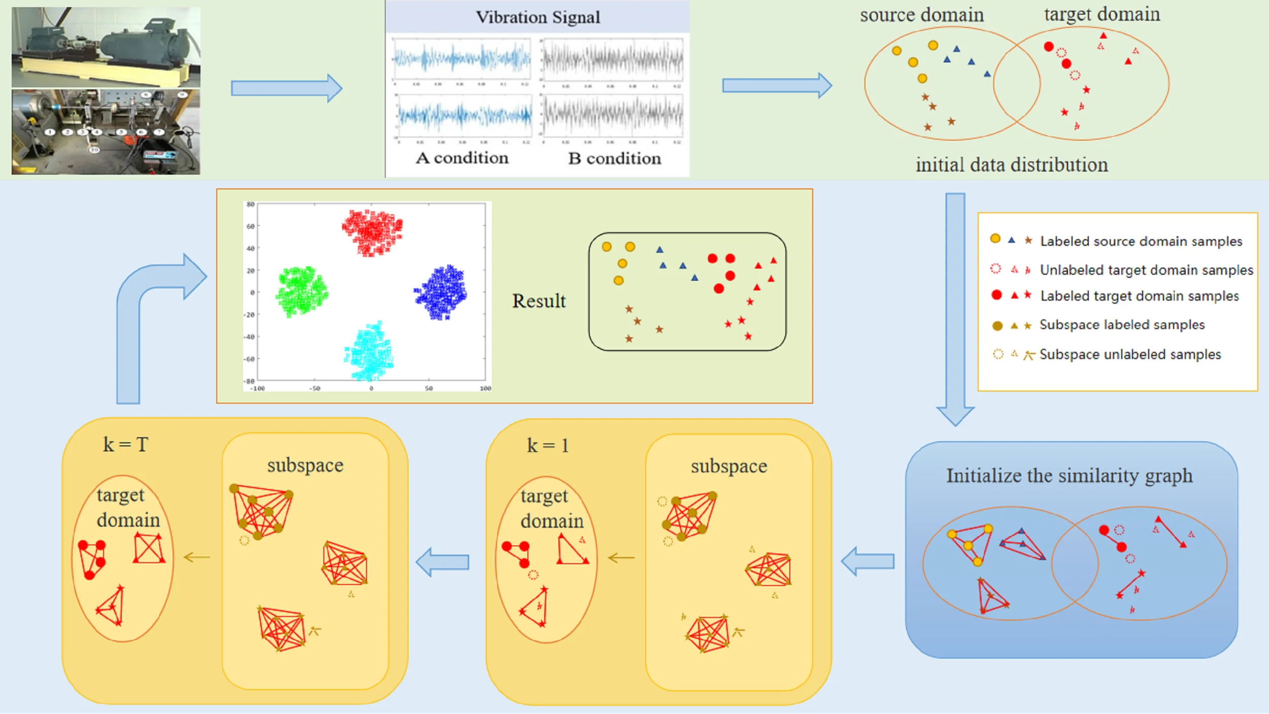
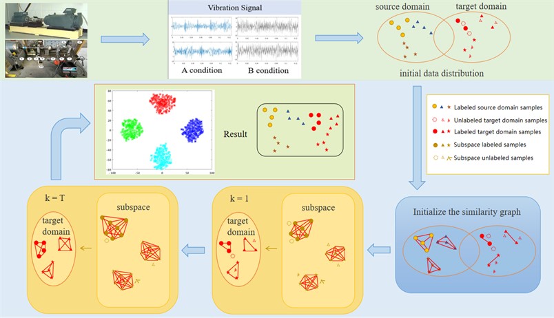
Based on cross-domain manifold structure preservation, low-dimensional data representation is established using the local neighborhood relationships between data samples. High-precision fault diagnosis for rolling bearings across various equipment was achieved in this study. Initially, similarity graphs were constructed separately for the source domain, target domain, and cross-domain. After that, the deterministic solution was obtained from the generalized eigenvalue problem. Mapping high-dimensional features into low-dimensional manifold subspaces preserves the nonlinear relationships between data. This alignment addresses differences in data distribution while maintaining the consistency in the cross-domain manifold structure. Additionally, the training dataset is updated with labeled target domain samples with higher confidence based on each mapping result. This promotes subspace learning in subsequent iterations and accurately identifies cross-machine fault samples. The overall flow chart of the model is shown in Fig. 1.

This investigation’s fault diagnosis approach unfolds in five pivotal stages:

Step 1: Vibration signals with identified labels from one machinery unit are designated as source domain $D_{s}$ , while signal data with unknown labels from a different apparatus are classified under target domain $D_{t}$ . Concurrently, a small subset of labeled samples from the target domain is designated as supervised samples $D_{t}^{l}$ . The feature extraction outcomes from vibration signals within both the source and the target domains serve as the foundational input.

Step 2: Based on the initial distribution of the samples, similarity graph matrices within both the source and target domains are initialized, establishing dimension $p$ and hyperparameter $α$ for the shared subspace.

Step 3: Solve the eigenvalues and eigenvectors of the generalized characteristic Eq. (13) to obtain the induced matrices $R_{s}$ and $R_{t}$ projected from the source and target domains to the low-dimensional manifold subspace.

Step 4: Update the sample distribution according to $Z_{s} = R_{s}^{T} X_{s}$ and $Z_{t} = R_{t}^{T} X_{t}$ , and use the $K$ -nearest neighbor ( $K =$ 1) to predict unlabeled samples in the target domain.

Step 5: Add samples with high confidence of the prediction results to the target domain supervised sample $D_{t}^{l}$ .

Repeat steps 3 through 5 until the results converge.

Fig. 1The overall process of the model

4. Experimental validation

To evaluate the proposed methodology’s efficacy and generalization capacity, this investigation employed fault data from two distinct testing apparatuses to assess the bearing fault diagnosis algorithm. The evaluation included bearing vibration data from Case Western Reserve University (CWRU) and a dataset produced by a bearing fault testing device constructed by our research group.

4.1. Dataset description

Dataset A: The first group of datasets was released by Case Western Reserve University, including bearing vibration data under four different working conditions (0 HP/1797 rpm, 1 HP/1772 rpm, 2 HP/1750 rpm, 3 HP/1730 rpm). For each working condition, the dataset records four health states of the bearing: normal (NO), outer ring fault (OF), inner ring fault (IF), and rolling element fault (BF). Additionally, the sampling frequency of the vibration signal is 12 kHz.

Dataset B: Originating from a custom-constructed experimental setup depicted in Fig. 2, this study's secondary dataset includes four distinct health conditions: normal operation (NO), outer ring defect (OF), inner ring defect (IF), and rolling element failure (BF). The examination involved three specific motor operational scenarios: a 500 N load at 1800 rpm, a 1000 N load at 1200 rpm, and a 1500 N load at 600 rpm, with a uniform sampling rate of 16 kHz across all data points.

Table 1Transfer task information of two datasets

Source domain				Target domain
Dataset	Working condition	Sampling frequency	Dataset	Working condition	Sampling frequency
A0	0 HP/1797 rpm	12 kHz	B1	500 N/1800 rpm	16 kHz
A0	0 HP/1797 rpm		B2	1000N/1200 rpm
A0	0 HP/1797 rpm		B3	1500 N/600 rpm
A1	1 HP/1772 rpm		B1	500 N/1800 rpm
A1	1 HP/1772 rpm		B2	1000N/1200rpm
A1	1 HP/1772 rpm		B3	1500 N/600 rpm
A2	2 HP/1750 rpm		B1	500 N/1800 rpm
A2	2 HP/1750 rpm		B2	1000N/1200 rpm
A2	2 HP/1750 rpm		B3	1500 N/600 rpm
A3	3 HP/1730 rpm		B1	500 N/1800 rpm
A3	3 HP/1730 rpm		B2	1000N/1200 rpm
A3	3 HP/1730 rpm		B3	1500 N/600 rpm

Fig. 2Self-built fault test rig: 1) motor; 2) coupling; 3) spindle; 4) bearing housing; 5) carbon brush; 6) test bearing housing; 7) vibration acceleration sensor; 8) bearing; 9) base; 10) power; 11) load bolts

Self-built fault test rig: 1) motor; 2) coupling; 3) spindle; 4) bearing housing; 5) carbon brush; 6) test bearing housing; 7) vibration acceleration sensor; 8) bearing; 9) base; 10) power; 11) load bolts

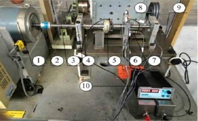
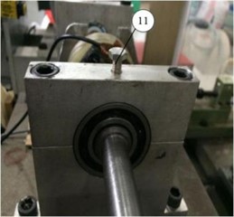
Table 2Type description of bearing dataset

Label	1	2	3	4
Type	NO	OF	IF	BF

This research establishes a framework for identifying faults in bearings across multiple devices. The methodology involves gathering vibration data from the bearings of any device operating under specified conditions, along with corresponding labels, to create a source domain dataset. Concurrently, data from a secondary device is acquired to develop a target domain dataset, aiming to replicate the process of identifying bearing fault types across different devices in real-world contexts. In this research, each health condition is represented by 100 samples, each containing 2048 data points, resulting in a total of 400 samples per dataset. This approach delineates migration tasks for fault diagnosis across 12 distinct devices. Details regarding the dataset are provided in Table 1, offering a comprehensive overview.

The datasets in Table 1 and Table 2, along with the signal spectrum in Fig. 3, facilitate a comprehensive analysis of signal spectra. This analysis reveals that frequency data for identical fault types shows substantial variations across different devices. These variations can compromise the efficiency of conventional fault diagnosis methodologies, leading to a significant decrease in the accuracy of bearing fault identification across different devices. Therefore, it is imperative to advance technologies for diagnosing faults in rolling bearings across multiple devices, highlighting their critical value for engineering applications.

Fig. 3Signal spectrum of fault dataset

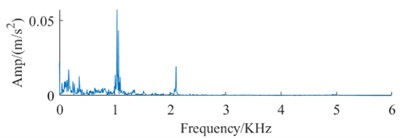
a) Spectrum of NO DataA

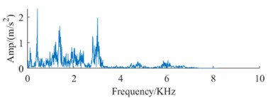
e) Spectrum of NO DataB

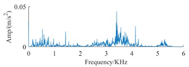
b) Spectrum of OF DataA

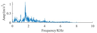
f) Spectrum of OF DataB

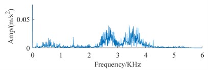
c) Spectrum of IF DataA

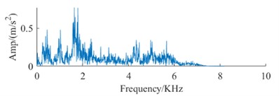
g) Spectrum of IF DataB

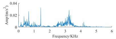
d) Spectrum of BF DataA

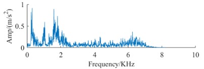
h) Spectrum of BF DataB

4.2. Experimental conclusion

To demonstrate the superior cross-domain transferability of CDMSP, this investigation conducts a comparative analysis with various machine learning algorithms. This examination includes three conventional machine learning algorithms and three prevalent transfer learning approaches, comprising two unsupervised and one semi-supervised methodology. A comprehensive description of each method is provided as follows:

KNN [3]: The K-nearest neighbor algorithm (KNN) is a benchmark method often used in classification tasks. In this study, the 1NN method ( $K =$ 1) is specifically used.

SVM [4]: The support vector machine (SVM) is another commonly used baseline algorithm in classification problems.

LPP [35]: Locality Preserving Mapping (LPP) is a manifold learning technique that maps high-dimensional data to low-dimensional space through nonlinear transformation. Its purpose is to maintain the nonlinear structural relationships between data points.

JDA [41]: Joint Distribution Adaptation (JDA) is an effective transfer learning technique that combines marginal distribution and conditional distribution adaptation.

MEDA [16]: Manifold Embedded Distribution Adaptation (MEDA) is an advanced transfer learning strategy that dynamically adjusts the weights of marginal and conditional distributions.

SSMTL [42]: Semi-Supervised Metric Transfer Learning (SSMTL) is a semi-supervised learning method with cross-domain metric ability, particularly suitable for transfer learning situations.

In the conducted research, the K-nearest neighbor algorithm (KNN, where $K =$ 1) was used as the fundamental classifier, with the shared subspace dimensionality set to 20 and the process iterated ten times. The hyperparameter B was set to 10.

Classification accuracy and the standard deviation accuracy of fault samples were used as metrics for evaluating algorithm performance. To validate the reliability of the outcomes, each task underwent 50 iterations, with the mean value of these iterations deemed the conclusive result. This approach facilitated the assessment of seven distinct classification algorithms’ efficacy in diagnosing bearing faults across various transfer tasks. The findings are presented in Table 3, which shows the diagnostic outcomes from transitioning the CWRU dataset to a proprietary bearing fault experimentation setup, highlighting the maximum recognition rate within identical tasks in bold.

To show the algorithm’s time complexity, we use the time required to complete the fault identification as the evaluation index. The unified operating environment is: Operating System: Windows 10; CPU: Intel (R) Core (TM) i7-12700H; GPU: NVIDIA GeForce RTX 3060; RAM: 16GB; Software: MATLAB 2019b.

Table 3Accuracy of bearing fault identification under different machines by different methods

Task	KNN	SVM	LPP	JDA	MEDA	SSMTL*	CDMSP*
A0→B1	38.25	33.00	53.75	49.00	50.00	85.53	100.00
A0→B2	41.00	28.25	18.25	49.50	49.50	83.68	100.00
A0→B3	22.50	18.50	30.50	48.25	49.50	82.63	95.27
A1→B1	41.25	44.25	42.25	50.00	50.00	87.11	100.00
A1→B2	39.25	32.25	23.00	50.00	50.00	88.95	100.00
A1→B3	18.75	25.50	29.75	47.75	29.25	77.37	94.84
A2→B1	43.00	53.50	48.00	50.00	50.00	88.16	100.00
A2→B2	45.25	40.00	49.00	50.00	50.00	90.79	100.00
A2→B3	29.00	24.25	23.00	48.50	31.25	83.16	94.13
A3→B1	51.50	55.50	30.50	50.00	50.00	88.16	100.00
A3→B2	48.75	35.25	44.00	50.00	50.00	87.11	99.70
A3→B3	33.75	24.75	22.50	48.75	32.75	73.42	94.92
Average	37.69	34.58	34.54	49.31	45.19	84.67	98.24
Std.	10.02	11.72	12.21	0.83	8.54	5.04	2.56
Time(s)	0.63	5.62	5.70	15.97	27.74	4.20	7.50
Note: The representation with * indicates semi-supervised transfer learning, which provides 1 % labeled samples of the target domain as supervised samples.

The analysis in Table 3 shows that the CDMSP methodology introduced in this investigation consistently outperforms six alternative fault diagnosis approaches across twelve cross-device fault diagnosis tasks, achieving superior fault detection accuracy in every evaluated task. The standard deviation and running time of 12 transfer task results indicate that CDMSP has excellent robustness and low time complexity.

In cross-machine fault diagnosis, the accuracy of traditional diagnostic models is only 30 %-40 %, and the accuracy of traditional transfer learning methods is also below 50 %. The SSMTL method, which provides supervised samples in the target domain, shows great improvement in fault identification across machine domains. Moreover, when the target domain data is a B3 transfer task, the fault identification accuracy of all methods is not high due to the target condition of low speed and heavy load, resulting in a greater distribution difference. This indicates that an elevated load can augment the spatial separation of bearing fault characteristics, consequently magnifying the variance in cross-domain distributions. When evaluating the efficacy of traditional classification algorithms in cross-device transfer tasks, it is observed that these tasks often yield suboptimal performance. Transfer learning emerges as a potent mechanism for mitigating such distributional disparities, enhancing task-specific accuracy, particularly through the application of semi-supervised transfer learning techniques, which in certain instances deliver superior detection outcomes. Nonetheless, the reliability of these techniques remains subpar, with certain tasks not achieving the requisite accuracy levels. This scenario underscores the complexities associated with diagnosing bearing faults across diverse machinery, compounded by the challenge of acquiring ample fault samples from operational machinery. Hence, leveraging insights from labeled data harvested from a single machine to facilitate intelligent fault diagnosis in other machinery holds significant practical implications.

4.3. Experimental analysis

4.3.1. Performance analysis of algorithms with limited supervised data

In engineering, the disparity in mechanical equipment’s operational environments significantly complicates the collection of bearing monitoring signals, often precluding the acquisition of adequate known-state bearing data samples. Consequently, this investigation seeks to assess the CDMSP algorithm's capacity to maintain diagnostic accuracy across various labeled supervisory samples within the target domain. By modulating the number of supervisory samples, the study evaluates the algorithm's efficacy across twelve cross-device fault diagnostic tasks. To mitigate variability in experimental findings, each diagnostic task was subjected to fifty iterations. The outcomes of these investigations are depicted through box plots, as illustrated in Fig. 4.

Fig. 4The performance of CDMSP under small supervised samples

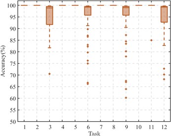
a) Number of supervised samples: 1

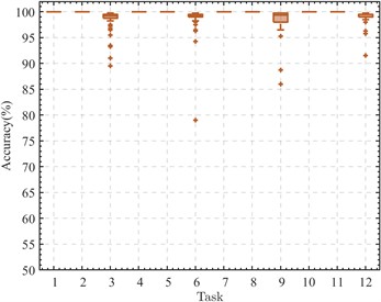
b) Number of supervised samples: 5

c) Number of supervised samples: 10

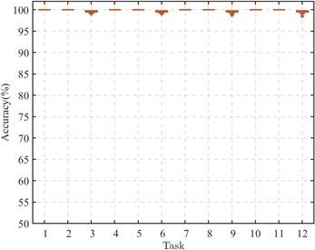
d) Number of supervised samples: 20

Analysis of the data in Fig. 3 indicates that, aside from transfer tasks targeting domain B3 (Tasks 3, 6, 9, 12), the CDMSP method demonstrates significant cross-device transfer proficiency even when supervised samples are scarce, with accuracy levels approaching 100 %. This evidences the method's robust performance in target operational conditions with low loads. However, when the target field's working condition is low speed and heavy load, the scarce supervision samples are insufficient to provide adequate cross-domain transfer information. When the number of supervised samples is 5, except for Task 6 (A1→B3) with an experimental accuracy rate of less than 80 %, other experimental results are greater than 85 %. When the number of supervised samples is greater than 10, the accuracy of CDMSP remains basically stable, proving that the distribution difference across machine domains is expanded due to excessive load, and more supervised samples are needed to improve cross-domain adaptive learning ability.

4.3.2. Diagnostic outcomes in the presence of noise disturbances

In the actual operation of rolling bearings, the external environment can interfere with the collected vibration signals. To evaluate the robustness of the CDMSP methodology under ambient noise conditions, test samples were deliberately infused with noise to mimic fault diagnosis environments influenced by such disturbances. Four distinct sets of cross-device fault identification tasks were randomly chosen, maintaining constant parameters within the diagnostic model. Noise intensities of 10 dB and 20 dB were subsequently introduced into the designated test samples. For result validation, each task underwent 50 iterations. The experimental results are illustrated in Fig. 5.

Fig. 4 shows that the CDMSP approach exhibits significant robustness in noisy environments, where the precision of fault detection remains largely unaffected by substantial noise disturbances. In particular, the three transfer tasks of A0 to B1, A0 to B2, and A1 to B1 are essentially not disturbed by noise, reflecting the robustness of CDMSP to noise. As mentioned earlier, the distributional difference across the machine domain caused by the excessive load of the target machine (task A0 to B3) is enlarged, reducing the accuracy of the diagnosis model. However, our method can still maintain high fault recognition accuracy in a noisy environment.

4.3.3. Subspace dimension and hyperparameter sensitivity analysis

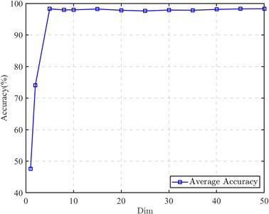
The primary goal of employing transfer learning to reduce variance in cross-domain distributions is to locate a shared subspace that minimizes the distance between domains. The CDMSP model uses projection matrices $R_{s}$ and $R_{t}$ to generate a reduced-dimensional manifold subspace. As detailed in Section 2, the dimensions of these projection matrices are specified as $d$ × $p$ , where $d$ is the dimensionality of the original sample space, and $p$ is the dimensionality of the shared subspace. This arrangement allows for a detailed exploration of which dimensions in the common subspace best retain domain-invariant features among diverse machine samples. Therefore, it is imperative to explore how changes in subspace dimensions impact the average efficacy of the CDMSP approach. Changing the dimensions of the projection matrices allows for the evaluation of average accuracy in different subspaces, as depicted in Fig. 6.

Examination of the findings in Fig. 6 reveals a significant increase in the recognition rate of the diagnostic model as subspace dimensionality increases from 1 to 5. Beyond this threshold, increasing the dimensionality from 5 to 50 does not significantly affect the model's average accuracy. This observation suggests that subspaces of insufficient dimensionality fail to capture cross-domain fault characteristics adequately, while maintaining lower dimensionality could significantly reduce further modeling costs. Thus, setting the dimensionality of CDMSP's shared subspace to exceed 5 is a prudent choice.

The CDMSP method proposed in this paper also includes another hyperparameter $α$ . As a regularization hyperparameter, we need to discuss its sensitivity in the model. $α = {0.0001, 0.001, 0.01, 0.1, 1, 10, 100, 1000}$ were set up respectively, and 50 experiments were conducted. The results are shown in Fig. 7.

Fig. 5The performance of CDMSP under noise

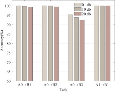
Fig. 6CDMSP in different dimensions

The average accuracy of each hyperparameter $α$ and its fluctuation range in repeated tests are shown in Fig. 7. When $α =$ 0.0001 or 0.001, the accuracy of CDMSP is low and unstable, often resulting in very low accuracy. When $α$ is greater than 0.01, the accuracy of the cross-domain fault identification model remains above 90 %. Therefore, $α$ should be set to a value greater than 0.01.

Fig. 7CDMSP at different α values

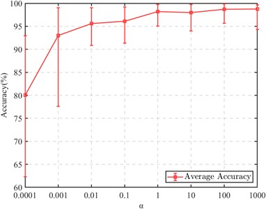
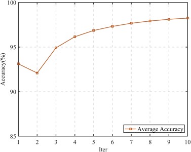
Fig. 8Diagnostic model convergence process

4.3.4. Analysis of model convergence

To study the convergence performance of CDMSP after cross-domain structure expansion, we present the changes in average fault identification accuracy from the CWRU data set to the self-built test rig data set. The results are shown in Fig. 8.

It is observed that as the number of iterations increases, the average recognition accuracy of CDMSP also increases. Although the accuracy decreases in the second iteration, a subspace with higher accuracy is learned in subsequent iterations, demonstrating CDMSP's good adaptive ability and convergence.

4.3.5. Analysis of feature visualization

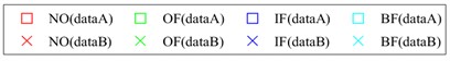
To enhance the understanding of sample distributions within the shared subspace, we visualized fault type distributions for the cross-machine transfer fault identification task A0→B3 using the t-distributed Stochastic Neighbor Embedding (t-SNE) algorithm [43]. The adaptation outcomes for four diagnostic models-KNN, LPP, SSMTL, and CDMSP-were represented using two-dimensional scatter plots. As shown in Fig. 9, markers with identical colors but different shapes indicated the same fault types, providing clearer visibility into the effectiveness of minimizing cross-domain distributions.

Examination of Fig. 9 shows notable distribution differences between the source and target domains in the initial distribution, with substantial overlap across diverse fault types. The use of conventional machine learning algorithms for fault diagnosis in such scenarios could lead to misclassification among distinct fault categories, resulting in extremely low model accuracy. After manifold projection, the cross-domain distribution difference in LPP is significantly reduced, but due to the lack of cross-domain adaptive ability, distinguishing between different categories remains difficult. The semi-supervised transfer learning method SSMTL increases discrimination between categories after adding cross-domain supervised samples, but the difference between cross-machine domains is not effectively reduced. The cross-domain manifold structure maintenance method proposed in this paper performs well in visualizing sample distribution. The inter-sample distribution distance among identical fault categories is significantly diminished, reducing cross-domain discrepancies. The inter-sample distribution distance among identical fault categories is significantly diminished, reducing cross-domain discrepancies.

Fig. 9A0→B3 bearing sample distribution two-dimensional scatter plot

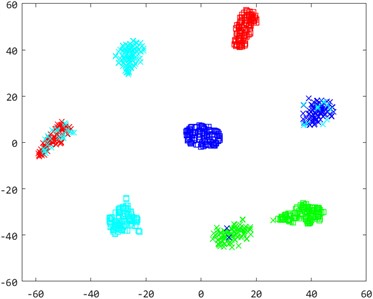
a) KNN

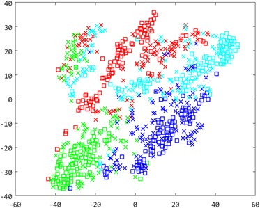
b) LPP

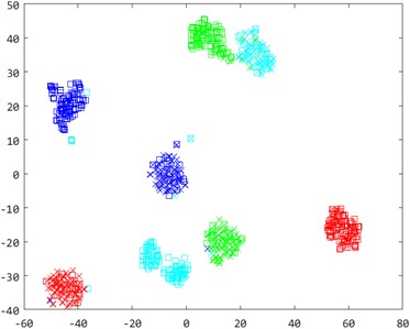
c) SSMTL

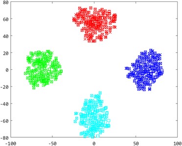
d) CDMSP

5. Conclusions

This paper proposes a cross-domain manifold structure-preserving method for cross-machine fault diagnosis. The CDMSP method expands the application of locality-preserving projection in the cross-machine domain. By introducing a cross-domain similarity graph, the generalized eigenvalue problem is solved to obtain a deterministic solution, establishing a local low-dimensional representation between the cross-machine domain data samples. High-dimensional features are mapped to a low-dimensional manifold subspace, preserving the nonlinear relationships between the data and maintaining the consistency of the cross-domain manifold structure while aligning data distribution differences. Experimental results on 12 cross-machine fault diagnosis tasks show that CDMSP has low time complexity, high fault identification accuracy, strong convergence, and excellent diagnostic performance on small load target equipment with sparsely labeled target samples. Additionally, the proposed method is not sensitive to hyperparameters, making it easy to select optimal hyperparameter values for different target machines or conditions. Therefore, CDMSP has a high practical application value in identifying faults in rolling bearings across different machines.

In future work, we will explore the application of CDMSP in a wider range of machines and more complex working conditions. This includes identifying more fault types and applying the method to unbalanced fault samples. Additionally, addressing the limitation that a few supervised samples are needed for CDMSP is a primary research direction.

References

J. Liu, C. Zhang, and X. Jiang, “Imbalanced fault diagnosis of rolling bearing using improved MsR-GAN and feature enhancement-driven CapsNet,” Mechanical Systems and Signal Processing, Vol. 168, p. 108664, Apr. 2022, https://doi.org/10.1016/j.ymssp.2021.108664

Publisher
S. Liu, H. Jiang, Z. Wu, and X. Li, “Data synthesis using deep feature enhanced generative adversarial networks for rolling bearing imbalanced fault diagnosis,” Mechanical Systems and Signal Processing, Vol. 163, p. 108139, Jan. 2022, https://doi.org/10.1016/j.ymssp.2021.108139

Publisher
D. Wang, “K-nearest neighbors based methods for identification of different gear crack levels under different motor speeds and loads: Revisited,” Mechanical Systems and Signal Processing, Vol. 70-71, pp. 201–208, Mar. 2016, https://doi.org/10.1016/j.ymssp.2015.10.007

Publisher
W. Mao, M. Tian, and G. Yan, “Research of load identification based on multiple-input multiple-output SVM model selection,” Proceedings of the Institution of Mechanical Engineers, Part C: Journal of Mechanical Engineering Science, Vol. 226, No. 5, pp. 1395–1409, Oct. 2011, https://doi.org/10.1177/0954406211423454

Publisher
S. R. Safavian and D. Landgrebe, “A survey of decision tree classifier methodology,” IEEE Transactions on Systems, Man, and Cybernetics, Vol. 21, No. 3, pp. 660–674, Jan. 1991, https://doi.org/10.1109/21.97458

Publisher
J. Jiao, M. Zhao, J. Lin, and K. Liang, “A comprehensive review on convolutional neural network in machine fault diagnosis,” Neurocomputing, Vol. 417, pp. 36–63, Dec. 2020, https://doi.org/10.1016/j.neucom.2020.07.088

Publisher
W. Zhao et al., “Multiscale inverted residual convolutional neural network for intelligent diagnosis of bearings under variable load condition,” Measurement, Vol. 188, p. 110511, Jan. 2022, https://doi.org/10.1016/j.measurement.2021.110511

Publisher
Y. Deng, D. Huang, S. Du, G. Li, C. Zhao, and J. Lv, “A double-layer attention based adversarial network for partial transfer learning in machinery fault diagnosis,” Computers in Industry, Vol. 127, p. 103399, May 2021, https://doi.org/10.1016/j.compind.2021.103399

Publisher
Y. Peng, F. Qin, W. Kong, Y. Ge, F. Nie, and A. Cichocki, “GFIL: a unified framework for the importance analysis of features, frequency bands, and channels in EEG-based emotion recognition,” IEEE Transactions on Cognitive and Developmental Systems, Vol. 14, No. 3, pp. 935–947, Sep. 2022, https://doi.org/10.1109/tcds.2021.3082803

Publisher
Y. Lei, B. Yang, X. Jiang, F. Jia, N. Li, and A. K. Nandi, “Applications of machine learning to machine fault diagnosis: A review and roadmap,” Mechanical Systems and Signal Processing, Vol. 138, p. 106587, Apr. 2020, https://doi.org/10.1016/j.ymssp.2019.106587

Publisher
T. Sun, G. Yu, M. Gao, L. Zhao, C. Bai, and W. Yang, “Fault diagnosis methods based on machine learning and its applications for wind turbines: a review,” IEEE Access, Vol. 9, pp. 147481–147511, Jan. 2021, https://doi.org/10.1109/access.2021.3124025

Publisher
G. Wang, S. Zhao, J. Chen, and Z. Zhong, “A novel compound fault diagnosis method for rolling bearings based on graph label manifold metric transfer,” Measurement Science and Technology, Vol. 34, No. 6, p. 065010, Jun. 2023, https://doi.org/10.1088/1361-6501/acbc39

Publisher
Y. A. Yucesan, A. Dourado, and F. A. C. Viana, “A survey of modeling for prognosis and health management of industrial equipment,” Advanced Engineering Informatics, Vol. 50, p. 101404, Oct. 2021, https://doi.org/10.1016/j.aei.2021.101404

Publisher
J. Li, R. Huang, J. Chen, J. Xia, Z. Chen, and W. Li, “Deep self-supervised domain adaptation network for fault diagnosis of rotating machine with unlabeled data,” IEEE Transactions on Instrumentation and Measurement, Vol. 71, pp. 1–9, Jan. 2022, https://doi.org/10.1109/tim.2022.3164136

Publisher
Z. Wang, X. He, B. Yang, and N. Li, “Subdomain adaptation transfer learning network for fault diagnosis of roller bearings,” IEEE Transactions on Industrial Electronics, Vol. 69, No. 8, pp. 8430–8439, Aug. 2022, https://doi.org/10.1109/tie.2021.3108726

Publisher
J. Wang, W. Feng, Y. Chen, H. Yu, M. Huang, and P. S. Yu, “Visual Domain Adaptation with Manifold Embedded Distribution Alignment,” in MM’18: ACM Multimedia Conference, pp. 402–10, Oct. 2018, https://doi.org/10.1145/3240508.3240512

Publisher
Z. Zhang, H. Chen, S. Li, Z. An, and J. Wang, “A novel geodesic flow kernel based domain adaptation approach for intelligent fault diagnosis under varying working condition,” Neurocomputing, Vol. 376, pp. 54–64, Feb. 2020, https://doi.org/10.1016/j.neucom.2019.09.081

Publisher
H. Shi, Y. Shang, X. Zhang, and Y. Tang, “Research on the initial fault prediction method of rolling bearings based on DCAE-TCN transfer learning,” Shock and Vibration, Vol. 2021, pp. 1–15, Mar. 2021, https://doi.org/10.1155/2021/5587756

Publisher
Z. Wu, H. Jiang, K. Zhao, and X. Li, “An adaptive deep transfer learning method for bearing fault diagnosis,” Measurement, Vol. 151, p. 107227, Feb. 2020, https://doi.org/10.1016/j.measurement.2019.107227

Publisher
Y. Zou, Y. Liu, J. Deng, Y. Jiang, and W. Zhang, “A novel transfer learning method for bearing fault diagnosis under different working conditions,” Measurement, Vol. 171, p. 108767, Feb. 2021, https://doi.org/10.1016/j.measurement.2020.108767

Publisher
S. Xing, Y. Lei, B. Yang, and N. Lu, “Adaptive knowledge transfer by continual weighted updating of filter kernels for few-shot fault diagnosis of machines,” IEEE Transactions on Industrial Electronics, Vol. 69, No. 2, pp. 1968–1976, Feb. 2022, https://doi.org/10.1109/tie.2021.3063975

Publisher
S. Luo, X. Huang, Y. Wang, R. Luo, and Q. Zhou, “Transfer learning based on improved stacked autoencoder for bearing fault diagnosis,” Knowledge-Based Systems, Vol. 256, p. 109846, Nov. 2022, https://doi.org/10.1016/j.knosys.2022.109846

Publisher
S. Wan, J. Liu, X. Li, Y. Zhang, K. Yan, and J. Hong, “Transfer-learning-based bearing fault diagnosis between different machines: A multi-level adaptation network based on layered decoding and attention mechanism,” Measurement, Vol. 203, p. 111996, Nov. 2022, https://doi.org/10.1016/j.measurement.2022.111996

Publisher
P. Xia, Y. Huang, Y. Wang, C. Liu, and J. Liu, “Augmentation-based discriminative meta-learning for cross-machine few-shot fault diagnosis,” Science China Technological Sciences, Vol. 66, No. 6, pp. 1698–1716, May 2023, https://doi.org/10.1007/s11431-022-2380-0

Publisher
Z. He, H. Shao, Z. Ding, H. Jiang, and J. Cheng, “Modified deep autoencoder driven by multisource parameters for fault transfer prognosis of aeroengine,” IEEE Transactions on Industrial Electronics, Vol. 69, No. 1, pp. 845–855, Jan. 2022, https://doi.org/10.1109/tie.2021.3050382

Publisher
S. Jia, Y. Deng, J. Lv, S. Du, and Z. Xie, “Joint distribution adaptation with diverse feature aggregation: A new transfer learning framework for bearing diagnosis across different machines,” Measurement, Vol. 187, p. 110332, Jan. 2022, https://doi.org/10.1016/j.measurement.2021.110332

Publisher
S. Xiang, J. Zhang, H. Gao, D. Shi, and L. Chen, “A deep transfer learning method for bearing fault diagnosis based on domain separation and adversarial learning,” Shock and Vibration, Vol. 2021, pp. 1–9, Jun. 2021, https://doi.org/10.1155/2021/5540084

Publisher
Q. Li, “A comprehensive survey of sparse regularization: fundamental, state-of-the-art methodologies and applications on fault diagnosis,” Expert Systems with Applications, Vol. 229, p. 120517, Nov. 2023, https://doi.org/10.1016/j.eswa.2023.120517

Publisher
Q. Li, “New sparse regularization approach for extracting transient impulses from fault vibration signal of rotating machinery,” Mechanical Systems and Signal Processing, Vol. 209, p. 111101, Mar. 2024, https://doi.org/10.1016/j.ymssp.2023.111101

Publisher
Z. Zhang et al., “Bearing fault diagnosis via generalized logarithm sparse regularization,” Mechanical Systems and Signal Processing, Vol. 167, p. 108576, Mar. 2022, https://doi.org/10.1016/j.ymssp.2021.108576

Publisher
L. Yu, C. Wang, F. Zhang, and H. Luo, “Bearing fault diagnosis via stepwise sparse regularization with an adaptive sparse dictionary,” Sensors, Vol. 24, No. 8, p. 2445, Apr. 2024, https://doi.org/10.3390/s24082445

Publisher
Z. Sun, Y. Wang, and J. Gao, “Intelligent fault diagnosis of rotating machinery under varying working conditions with global-local neighborhood and sparse graphs embedding deep regularized autoencoder,” Engineering Applications of Artificial Intelligence, Vol. 124, p. 106590, Sep. 2023, https://doi.org/10.1016/j.engappai.2023.106590

Publisher
F. Pancaldi, L. Dibiase, and M. Cocconcelli, “Impact of noise model on the performance of algorithms for fault diagnosis in rolling bearings,” Mechanical Systems and Signal Processing, Vol. 188, p. 109975, Apr. 2023, https://doi.org/10.1016/j.ymssp.2022.109975

Publisher
K. Zhang, C. Fan, X. Zhang, H. Shi, and S. Li, “A hybrid deep-learning model for fault diagnosis of rolling bearings in strong noise environments,” Measurement Science and Technology, Vol. 33, No. 6, p. 065103, Jun. 2022, https://doi.org/10.1088/1361-6501/ac4a18

Publisher
Q. Wang and F. Xu, “A novel rolling bearing fault diagnosis method based on adaptive denoising convolutional neural network under noise background,” Measurement, Vol. 218, p. 113209, Aug. 2023, https://doi.org/10.1016/j.measurement.2023.113209

Publisher
Z. Shao, W. Li, H. Xiang, S. Yang, and Z. Weng, “Fault diagnosis method and application based on multi-scale neural network and data enhancement for strong noise,” Journal of Vibration Engineering and Technologies, Vol. 12, No. 1, pp. 295–308, Jan. 2023, https://doi.org/10.1007/s42417-022-00844-x

Publisher
P. Lyu, K. Zhang, W. Yu, B. Wang, and C. Liu, “A novel RSG-based intelligent bearing fault diagnosis method for motors in high-noise industrial environment,” Advanced Engineering Informatics, Vol. 52, p. 101564, Apr. 2022, https://doi.org/10.1016/j.aei.2022.101564

Publisher
S. Gong, K. Xing, A. Cichocki, and J. Li, “Deep learning in EEG: advance of the last ten-year critical period,” IEEE Transactions on Cognitive and Developmental Systems, Vol. 14, No. 2, pp. 348–365, Jun. 2022, https://doi.org/10.1109/tcds.2021.3079712

Publisher
X. He and P. Niyogi, “Locality preserving projections,” Advances in Neural Information Processing Systems, Vol. 16, pp. 153–160, 2003.

Search CrossRef
K. S. Mcclure, R. B. Gopaluni, T. Chmelyk, D. Marshman, and S. L. Shah, “Nonlinear process monitoring using supervised locally linear embedding projection,” Industrial and Engineering Chemistry Research, Vol. 53, No. 13, pp. 5205–5216, Apr. 2014, https://doi.org/10.1021/ie401556r

Publisher
M. Long, J. Wang, G. Ding, J. Sun, and P. S. Yu, “Transfer feature learning with joint distribution adaptation,” in IEEE International Conference on Computer Vision (ICCV), Dec. 2013, https://doi.org/10.1109/iccv.2013.274

Publisher
R. K. Sanodiya and J. Mathew, “A framework for semi-supervised metric transfer learning on manifolds,” Knowledge-Based Systems, Vol. 176, pp. 1–14, Jul. 2019, https://doi.org/10.1016/j.knosys.2019.03.021

Publisher
L. van der Maaten and G. Hinton, “Visualizing data using t-SNE,” Journal of Machine Learning Research, Vol. 9, No. 11, pp. 2579–2605, 2008.

Search CrossRef

About this article

Received

10 March 2024

Accepted

03 July 2024

Published

22 August 2024

SUBJECTS

Fault diagnosis based on vibration signal analysis

DOI

https://doi.org/10.21595/jve.2024.24067

Keywords

bearing fault diagnosis

transferable

structure preservation

cross-machine

Acknowledgements

This study was supported by the Guangdong Provincial Foundation for Basic and Applied Basic Research (offshore wind power) (Project No. 2022A515240043), Guangdong Provincial Natural Science Foundation (Project No. 2023A1515012698), the National Key R&D Program of China (Project No. 2023YFB3406100), and the 2023 Zhanjiang Science and Technology Development Special Fund Competitive Allocation Project (No. 2023A216-32).

Data Availability

The datasets generated during and/or analyzed during the current study are available from the corresponding author on reasonable request.

Author Contributions

Can Li: conceptualization, data curation, methodology, software, validation, writing-original draft preparation. Guangbin Wang: conceptualization, formal analysis, funding acquisition, investigation, project administration, resources, writing-review and editing. Shubiao Zhao: conceptualization, visualization, writing-original draft preparation. Zhixian Zhong: funding acquisition, formal analysis, project administration, supervision. Ying Lv: funding acquisition, project administration, writing-review and editing.

Conflict of interest

The authors declare that they have no conflict of interest.

This is an open access article distributed under the Creative Commons Attribution License, which permits unrestricted use, distribution, and reproduction in any medium, provided the original work is properly cited.

Previous article in issue Previous Next article in issue Next

Research article

2024 01 21

Rolling bearing fault diagnosis based on variational mode decomposition and weighted multidimensional feature entropy fusion

Na Lei, Feihu Huang, Chunhui Li

Research article

2023 10 30

Cross domain fault diagnosis method based on MLP-mixer network

Xiaodong Mao

Research article

2023 09 08

Research on fault diagnosis method of bearing based on parameter optimization VMD and improved DBN

Yingqian Sun, Zhenzhen Jin

Research article

2023 08 18

Fault diagnosis of rolling bearing based on cross-domain divergence alignment and intra-domain distribution alienation

Shubiao Zhao, Guangbin Wang, Xuejun Li, Jinhua Chen, Lingli Jiang

C. Li, G. Wang, S. Zhao, Z. Zhong, and Y. Lv, “Cross-domain manifold structure preservation for transferable and cross-machine fault diagnosis,” Journal of Vibroengineering, Vol. 26, No. 6, pp. 1367–1384, Aug. 2024, https://doi.org/10.21595/jve.2024.24067

Copy Extrica

Copied to clipboard!

TY  - JOUR
DO  - 10.21595/jve.2024.24067
UR  - https://doi.org/10.21595/jve.2024.24067
TI  - Cross-domain manifold structure preservation for transferable and cross-machine fault diagnosis
T2  - Journal of Vibroengineering
AU  - Li, Can
AU  - Wang, Guangbin
AU  - Zhao, Shubiao
AU  - Zhong, Zhixian
AU  - Lv, Ying
PY  - 2024
DA  - 2024/08/22
PB  - Extrica
SP  - 1367-1384
VL  - 26
IS  - 6
SN  - 1392-8716
SN  - 2538-8460
ER  - 

Copy Ris

Copied to clipboard!

 @article{Li_2024, title={Cross-domain manifold structure preservation for transferable and cross-machine fault diagnosis}, ISSN={2538-8460}, url={https://doi.org/10.21595/jve.2024.24067}, DOI={10.21595/jve.2024.24067}, journal={Journal of Vibroengineering}, publisher={JVE International Ltd.}, author={Li, Can and Wang, Guangbin and Zhao, Shubiao and Zhong, Zhixian and Lv, Ying}, year={2024}, month=aug }

Copy Bibtex

Copied to clipboard!

[1]C. Li, G. Wang, S. Zhao, Z. Zhong, and Y. Lv, “Cross-domain manifold structure preservation for transferable and cross-machine fault diagnosis,” Journal of Vibroengineering, Aug. 2024, doi: 10.21595/jve.2024.24067.

Copy IEEE

Copied to clipboard!

Li, Can, Guangbin Wang, Shubiao Zhao, Zhixian Zhong, and Ying Lv. “Cross-Domain Manifold Structure Preservation for Transferable and Cross-Machine Fault Diagnosis.” Journal of Vibroengineering, August 22, 2024. https://doi.org/10.21595/jve.2024.24067.

Copy Chicago

Copied to clipboard!

Cross-domain manifold structure preservation for transferable and cross-machine fault diagnosis

Abstract

Highlights

1. Introduction

2. Cross-domain manifold structure preservation

2.1. Locality preserving projections

2.2. Cross-domain manifold structure preservation

3. Cross-domain manifold structure preservation-based fault diagnosis model for rolling bearings across machines

4. Experimental validation

4.1. Dataset description

4.2. Experimental conclusion

4.3. Experimental analysis

4.3.1. Performance analysis of algorithms with limited supervised data

4.3.2. Diagnostic outcomes in the presence of noise disturbances

4.3.3. Subspace dimension and hyperparameter sensitivity analysis

4.3.4. Analysis of model convergence

4.3.5. Analysis of feature visualization

5. Conclusions

References

About this article

Related Articles