Abstract
In the application of ultrasonic guided wave testing for rail crack detection, it is necessary to select a guided wave mode that is more sensitive to cracks as the detection mode. However, ultrasonic guided waves have multi-mode and dispersive characteristics. In order to extract mode information from complex signals, this paper proposes an optimal detection mode selection method based on the sensitivity of guided wave modes to cracks. This method is different from the traditional method of determining mode types by calculating the mode velocity through the arrival time of wave packets in the time domain signal. Based on the dispersion characteristics and mode features of guided wave modes, this paper establishes a crack sensitivity evaluation index. In a wide frequency band and among numerous modes, the guided wave modes suitable for detecting cracks in different regions of the full cross-section of rails are accurately selected. Experimental results show that the guided wave modes selected by the mode selection method proposed in this paper, based on the crack area energy and crack reflection intensity evaluation indexes, can accurately identify rail cracks, laying a foundation for the research on rail crack detection and localization methods.
1. Introduction
Detecting cracks across the full cross-section of rails is an international challenge. In the study of rail crack detection methods, ultrasonic bulk wave detection has high sensitivity to rail cracks but cannot achieve long-distance inspection of the full cross-section of rails. Magnetic particle testing, eddy current testing, magnetic flux leakage testing, radiographic testing, and machine vision testing can only detect surface or near-surface cracks on rails and cannot detect internal cracks. Acoustic emission and ultrasonic guided wave testing are fixed detection methods that can achieve long-distance detection of cracks. Among them, although acoustic emission can detect cracks across the full cross-section of rails, the research is limited to the detection of new or developing damage and cannot identify existing stable damage, and is greatly affected by external environmental noise [1]. In comparison, ultrasonic guided waves have the advantages of long propagation distance, fast speed, and wide coverage range. The guided wave transducer can be permanently fixed on the rail without affecting the normal operation of trains, making it suitable for detecting cracks in the full cross-section of rails and for all-weather online monitoring [2, 3].
Ultrasonic guided waves can cover the entire cross-section of rails, overcoming the detection blind spots in other non-destructive testing methods. At the same time, ultrasonic guided waves propagate over long distances, with fast propagation speeds and high detection efficiency, making them suitable for long-distance rail crack detection. The detection process does not require the train to stop, and through long-term fixation on the rail, it can achieve full cross-section, all-weather online monitoring of cracks [4-6], with good application prospects and research value. When using ultrasonic guided waves to detect rail cracks, it is necessary to select guided wave modes that are more sensitive to cracks as the detection modes. There are many types of modes that can propagate in rails, and as the frequency increases, more types of modes can be excited inside the rail. The increasing number of modes makes crack detection more difficult. In order to extract mode information from complex signals, researchers at home and abroad have studied various identification methods, mainly including time-domain signal methods [7-9], short-time Fourier transform methods [10-12], and single-mode extraction algorithms [13-15].
The time-domain signal method is more suitable for the analysis of signals with simple mode components and is often used as a method to determine whether the target mode exists in research work, but it is not suitable for analyzing complex signals with multiple modes. When the frequency components in the signal are relatively complex, considering the resolution and integrity of information, high-frequency components require a narrower time window, and low-frequency components require the opposite. Due to the inability of the short-time Fourier transform method to simultaneously satisfy the time and frequency resolutions of high-frequency and low-frequency components, the single-mode extraction algorithm can be applied to crack detection in rails. However, this method is only suitable for cases where mode identification is required. Since the detection process requires collecting a large amount of received signals, the operation is relatively complex, and it is currently less used.
Based on this, this paper proposes an optimal detection mode selection method based on the sensitivity of guided wave modes to cracks, focusing on the rail head. Based on the position and trend of crack generation, energy and reflection intensity indexes of crack area are established. Among numerous modes in a wide frequency band, guided wave modes suitable for detecting cracks in different regions of the full cross-section of rails are accurately selected, ultimately achieving the optimal selection of detection modes for cracks in the rail head region.
2. Algorithm for evaluating the crack sensitivity of guided wave modes
The wavelength of guided waves can impact the accuracy of crack detection. When the frequency of guided waves is low, their wavelength is relatively long, resulting in lower precision in crack detection. Therefore, for damage detection using guided waves, ultrasonic waves with frequencies greater than 20 kHz are typically employed. However, when the frequency of guided waves in railway tracks exceeds 60 kHz, the distribution of modal vibrations tends to favor surface waves, which is disadvantageous for detecting internal cracks in railway tracks. To ensure the applicability of the evaluation method to cracks across the entire cross-section of railway tracks while considering both detection accuracy and signal analysis complexity, this paper confines the frequency range to between 20 kHz and 60 kHz.
The detection of cracks in railway tracks using ultrasonic guided waves involves analyzing the echo signals generated by the interaction of cracks with guided wave modes to achieve crack localization. Given that the same crack affects different modes to varying degrees, this paper employs modal crack zone energy and modal crack reflection intensity as evaluation indicators for the crack sensitivity of guided wave modes. The crack sensitivity, denoted by Sc, is defined to characterize the extent to which cracks interact with different modes, as shown in Eq. (1):
where, Sre stands for the energy of the modal crack zone, and Sri represents the quantity of evaluation indicators for the mechanism of modal crack reflection intensity.
2.1. Evaluation indicator for modal crack zone energy
Research indicates that when applying ultrasonic guided waves to detect specific location cracks in railway tracks, the guided wave modes with more pronounced vibrations at the crack location exhibit higher sensitivity to the crack. It is common to select modes with larger amplitudes at the crack location and smaller amplitudes at other locations for detection. In this paper, we define the evaluation indicator Sre, representing the energy of the modal crack zone, to characterize the vibrations of various modes near the crack location. The rail section is divided into 255 units and 177 nodes, as illustrated in Fig. 1(a).
Fig. 1Rail cross-section mesh division and node selection
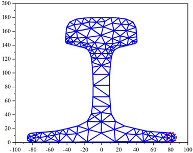
a) Rail cross-section mesh division
b) Node selection
Assuming the coordinates of the two endpoints of the crack are denoted as A(xA,yA) and B(xB,yB), according to Eq. (2), find the two nodes A'(xA',yA')and B'(xB',yB') on the cross-section closest to the crack endpoints. Here, Nall represents the number of nodes on the rail section:
Taking the midpoint between A' and B' as C'(xC',yC'), form a circle with C' as the center and r as the radius. As shown in Fig. 1(b), the rail section covered by the circle represents the selected crack zone, and the Noverlay nodes covered by the circle are the nodes chosen to characterize the energy magnitude of the crack zone. The node numbers are denoted as N1,N2,…,NNoverlay. Where:
According to the railway’s wave equation, solve the vibrational mode data for all nodes in each direction for each mode, denoted as MSDx(fi,N,mi), MSDy(fi,N,mi) and MSDz(fi,N,mi) respectively. Here, fi represents the frequency, mi is the mode index at frequency fi, and N is the node index. Then, for each mode, the average vibrational displacement of the nodes near the crack and all nodes on the cross-section is given by:
where, N=N1,N2,…,NNoverlay, and the corresponding modal zone energy is represented by Eq. (5). This equation is used to characterize the vibration and energy distribution states of each mode near the crack zone:
When the average vibrational displacement of nodes in the crack zone is significantly smaller than the average vibrational displacement of all nodes on the rail section (i.e., AVDnnc(fi)<AVDan(fi)), Sre(fi)<0. Conversely, when the average vibrational displacement of nodes in the crack zone is much larger than the average vibrational displacement of all nodes on the rail section (i.e., AVDnnc(fi)≫AVDan(fi)), Sre(fi) approaches 1. Normalize the results of Eq. (5) to obtain Sre(fi)∈[0,1]. From Eq. (5), it can be observed that when the coefficient Sre(fi) of the modal crack zone energy indicator is larger, the vibration of the mode in the crack zone is greater, indicating higher sensitivity to the crack. When Sre(fi) approaches 1, it signifies that the energy of the mode in the crack zone is significantly greater than the energy at other locations.
2.2. Evaluation indicator for modal crack reflection intensity
During the signal acquisition process in railway crack detection, the detection results can be influenced by the collection equipment and on-site noise. If the amplitude of the received crack echo signal is low, the risk of false negatives may occur. Therefore, modes with higher reflection echo amplitudes are more sensitive to cracks. When the vibration direction of the guided wave mode is orthogonal to the crack trend, the echo amplitude is greater than the mode with the vibration direction parallel to the crack trend. For modes where the vibration direction is neither orthogonal nor parallel to the crack trend, the amplitude falls between the two cases. Based on the vibration characteristics of the modes, this paper defines the evaluation indicator Sri for modal crack reflection intensity to characterize the degree of reflection when a mode encounters a crack. At frequency fi, the coefficient for the crack reflection intensity evaluation indicator of mode mi is given by:
where, Q represents the mode vibration direction vector, and P represents the crack trend direction vector. When the crack direction is orthogonal to the mode vibration direction, |Q⋅P|=0, and Sri(fi)=1. When the crack direction is parallel to the mode vibration direction, |Q⋅P| is maximized, and Sri(fi) is minimized. Therefore, as the value of Sri(fi) approaches 1, the orthogonality between the two improves, and the reflection wave from the crack becomes more pronounced. To prevent abrupt changes in the calculation results, it is necessary to add more nodes to the vector. According to the finite element discretization method, the vibrational mode
V at any point within a discretized element can be expressed in the form of shape functions:
In the equation, N(x,y) represents the shape function matrix, and q(e) represents the node vibrational vector:
In this equation, Ni represents the shape functions of the finite element unit.
At a frequency of fi, the vibrational mode mi at points A'(xA',yA') and B'(xB',yB') is denoted as VA' and VB' respectively. Divide the line segment between A' and B' into four equal parts, with the three intermediate points labeled as A'1(xA'1,yA'1), A'2(xA'2,yA'2), A'3(xA'3,yA'3). Given the vibrational data of the three nodes in the triangular element where the intermediate points are located, applying Eqs. (7-9), allows for the determination of the vibrational data VA'1, VA'2, VA'3 at these three intermediate points. This, along with VA' and VB', forms a new vibrational vector denoted as Q:
Similarly, divide the line segment between the crack points A and B into four equal parts, with the three intermediate points labeled as A1(xA1,yA1), A2(xA2,yA2), A3(xA3,yA3). This, along with points A and B, forms a coordinate vector denoted as P:
If the mode vibration direction is orthogonal to the crack trend, |Q⋅P|=0, Sri(fi)=1, and if the mode vibration direction is not orthogonal, |Q⋅P|>0, Sri(fi)<1. Normalize the results of Eq. (6) to obtain Sri(fi)∈[0,1]. Therefore, as the coefficient of the modal crack reflection intensity evaluation indicator approaches 1, the greater the orthogonality between the mode and the crack, the more pronounced the reflection when the mode encounters the crack.
In summary, the degree to which a crack affects guided wave modes is positively correlated with the size of the modal crack zone energy evaluation indicator. When the energy in the crack zone is relatively similar, a larger crack reflection intensity leads to higher echo amplitudes, indicating greater sensitivity of the mode to the crack.
3. Simulation analysis and experimental validation
3.1. Simulation analysis
To validate the evaluation criteria of crack area energy and crack reflection intensity for guided wave modes and to analyze their effects, this study focuses on analyzing the mechanism of cracks on guided wave modes using transverse cracks on rail heads as the research object. The correctness of the algorithm is verified through simulation and experimentation.
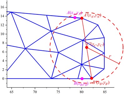
When guided waves propagate in rails, the number of modes increases significantly with frequency. When the frequency of guided waves exceeds 60 kHz, their distribution in the rail gradually tends towards surface waves, which is not conducive to detecting cracks across the entire rail section. Additionally, the fewer modes that can propagate in the rail, the easier the problem analysis becomes. However, at lower frequencies, guided waves have longer wavelengths, which can detect larger cracks but with lower accuracy. Therefore, considering both crack detection accuracy and the coverage of guided waves, the study focuses on the frequency range of [20, 60] kHz. The vibrational modes of guided waves in rails are calculated at frequencies of 20 kHz, 30 kHz, 40 kHz, 50 kHz, and 60 kHz, as shown in Fig. 2.
Fig. 2Mode shapes of guided waves in rails
As the frequency of guided waves increases from 20 kHz to 60 kHz, the number of propagating guided wave modes in the rail increases from 13 to 35, nearly doubling. While the increase in the selection space for modes is beneficial, the vibration patterns of the modes become more complex, leading to significantly increased research difficulty.
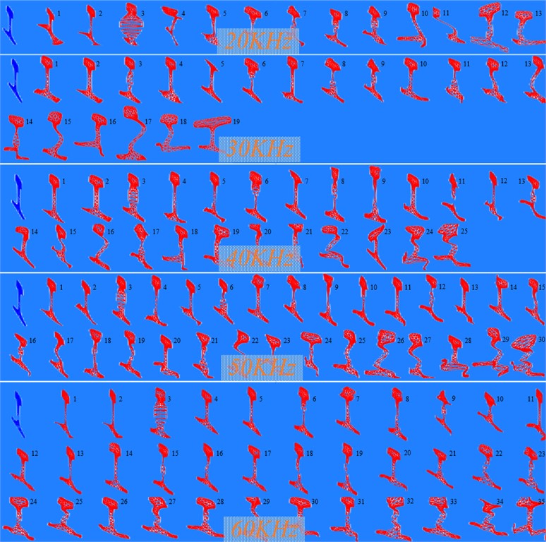
The positions of transverse cracks in the rail head are set as shown in Fig. 3. In this study, we assume points A and B coincide with points A' and B', located at nodes 109 and 117 on the cross-section. The longitudinal coordinates of the two ends of the crack are set to zero. Five frequency points are selected from the specified frequency range: 20 kHz, 30 kHz, 40 kHz, 50 kHz, and 60 kHz. Using the wave equation for the rail, we calculate the vibrational data for all modes at these five frequency points, totaling 122 modes. Using Eq. (5), we calculate the crack zone energy evaluation indicator Sre for all modes, as shown in Fig. 4. After sorting from largest to smallest, the first 20 modes (Sre) are listed in Table 1.
From Table 1, it can be seen that the 7th mode in the [40, 60] kHz range and the 5th mode at 30 kHz have the highest energy and the most pronounced vibration in the transverse crack area of the rail head. By examining the corresponding mode shapes in Fig. 2, it can be seen that these four modes are actually the same mode, all showing the most pronounced vibration in the rail head, which is consistent with the calculation results of the crack area energy evaluation criteria.
Fig. 3Transverse crack in rail head
Fig. 4Calculation results of modal crack zone energy indicator Sre
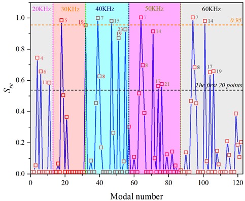
Table 1Calculated values of modal crack zone energy Sre for transverse crack in rail head
Frequency (kHz) | Modal number | Sre | Frequency (kHz) | Modal number | Sre |
2 | 4 | 0.74 | 5 | 7 | 1 |
6 | 0.64 | 8 | 0.69 | ||
11 | 0.57 | 14 | 0.91 | ||
3 | 5 | 0.98 | 17 | 0.55 | |
19 | 0.95 | 21 | 0.57 | ||
4 | 7 | 1 | 6 | 7 | 1 |
8 | 0.62 | 8 | 0.67 | ||
15 | 0.97 | 14 | 0.97 | ||
19 | 0.87 | 17 | 0.64 | ||
23 | 0.92 | 19 | 0.65 |
From the calculated results of the modal crack zone energy for transverse cracks in the rail head, modes corresponding to Sre∈[0.95,1] are selected. The crack reflection intensity evaluation indicator Sri is then calculated for each mode. After sorting the values in descending order, the results are presented in Table 2.
From Table 1-2, it can be observed that when the crack zone energy evaluation indicator Sre for transverse cracks in the rail head is equal to 1, the crack reflection intensity evaluation indicator Sri varies for different modes. Specifically, the crack reflection intensity for mode 7 at 60 kHz is approximately twice as large as that for mode 7 at 40 kHz. Therefore, among the 122 modes, the influence of transverse cracks in the rail head is relatively significant for mode 15 at 40 kHz, mode 5 at 30 kHz, mode 7 in the frequency range of 40 kHz to 60 kHz, mode 14 at 60 kHz, and mode 19 at 30 kHz.
Table 2Calculated values of crack reflection intensity Sri for transverse crack in rail head
Frequency (kHz) | Modal number | Sri |
4 | 15 | 0.96 |
3 | 5 | 0.75 |
6 | 7 | 0.61 |
5 | 7 | 0.49 |
4 | 7 | 0.31 |
6 | 14 | 0.21 |
3 | 19 | 0.19 |
For the mode 7 at 60 kHz, which has the maximum crack zone energy indicator Sre, a comparison is made with the mode 7 at 40 kHz, where the crack reflection intensity Sre is the same but differs by a factor of two. Similarly, to analyze the influence of crack zone energy indicator Sre on mode selection results, as well as the relationship between Sre and Sri, mode 1 at 50 kHz with Sre value of 0 but the maximum Sri value is selected for comparison. The crack zone energy evaluation indicators and reflection intensity evaluation indicators for these three modes are shown in Table 3.
Table 3Sensitivity parameters of modes
Frequency (kHz) | Modal number | Sre | Sri |
6 | 7 | 1 | 0.61 |
4 | 7 | 1 | 0.31 |
5 | 1 | 0 | 1 |
Establish a three-dimensional rail model with a length of 3.5 m. Set the grid width in the length direction of the rail to 3 mm according to Eqs. (2-21), with the crack located at 1.75 m, as shown in Fig. 5.
Fig. 5Transverse crack on the rail head
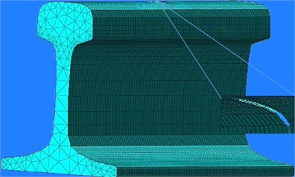
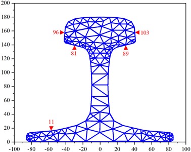
As per the configuration described by Lgrid≤λmin/10, the grid width along the length direction of the rail is set to 3 mm, and the crack is located at 1.75 m. An excitation is set at 0 m on the rail end, with an excitation signal being a sinusoidal wave modulated by a 5-cycle Hanning window. The central frequency is 60 kHz. A receiver is placed at 60 mm in the same direction, positioned at the same node as the excitation point. For the 60 kHz frequency, the 7th mode is excited vertically at nodes 81 and 89, and the signal is received at node 89. For the 40 kHz frequency, the 7th mode is excited vertically at nodes 96 and 103, and the signal is received at node 103. For the 50 kHz frequency, the 1st mode is excited and received at node 11, and the node positions are illustrated in Fig. 6.
Using the three-dimensional finite element simulation software ANSYS for calculations, the simulation duration was 3 ms, with a total of 3600 calculation steps. The simulation results are shown in Figs. 7-9.
Fig. 6Excitation and reception node locations
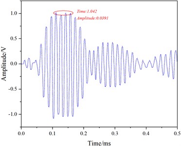
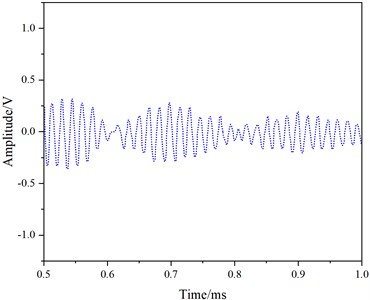
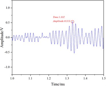
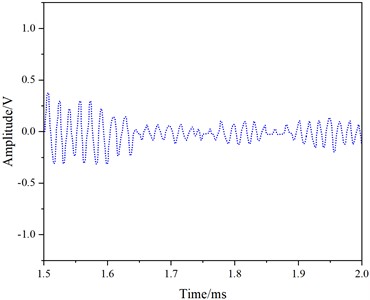
At 60 kHz frequency, Fig.7 illustrates the received and reflected waveforms for mode 7. The first waveform (Fig. 7(a)) corresponds to the direct wave received, the second waveform (Fig. 7(c)) represents the reflection from the rail bottom crack, and the third waveform (Fig. 7(e)) corresponds to the reflection from the rail end face. The distance (d) between the end face and the receiving position is 3.45 m. The peak time (t0) for the direct wave is 0.0624 ms, for the rail crack reflection time (t1) is 1.1135 ms with an amplitude of 0.00713 mm, and for the end face reflection time (t2) is 2.2254 ms.
Fig. 7Simulation results for mode 7 at a frequency of 60 kHz
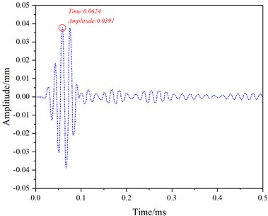
a) 0-0.5 ms
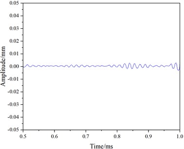
b) 0.5-1.0 ms
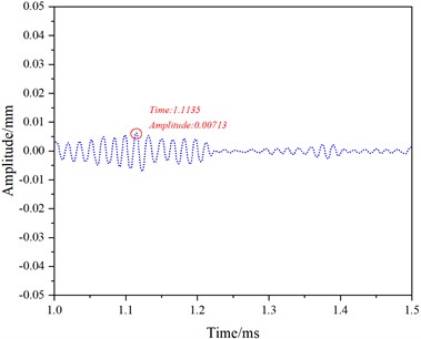
c) 1.0-1.5 ms
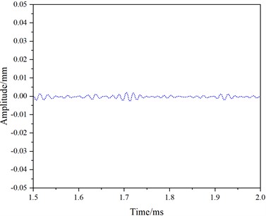
d) 1.5-2.0 ms
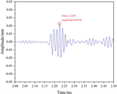
e) 2.0-2.5 ms
f) 2.5-3.0 ms
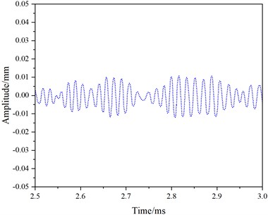
At a frequency of 40 kHz, Fig. 8 shows the received and reflected waveforms for mode 7. The first waveform (Fig. 8(a)) corresponds to the received direct wave, the second waveform (Fig. 8(c)) represents the reflection from the rail bottom crack, and the third waveform (Fig. 8(e)) corresponds to the reflection from the rail end face. The distance (d) between the end face and the receiving position is 3.45 m. The peak time (t0) for the direct wave is 0.1105 ms, for the rail crack reflection time (t1) is 1.1603 ms with an amplitude of 0.00713 mm, and for the end face reflection (t2) is 2.3246 ms.
Fig. 8depicts the simulation results for mode 7 at a frequency of 40 kHz over the time interval from 0 to 3 ms
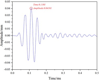
a) 0-0.5 ms
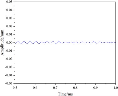
b) 0.5-1.0 ms
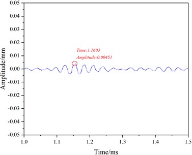
c) 1.0-1.5 ms
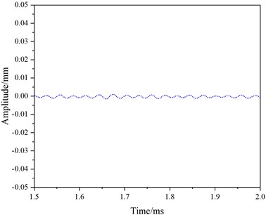
d) 1.5-2.0 ms
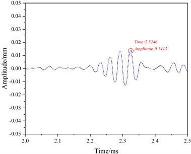
e) 2.0-2.5 ms
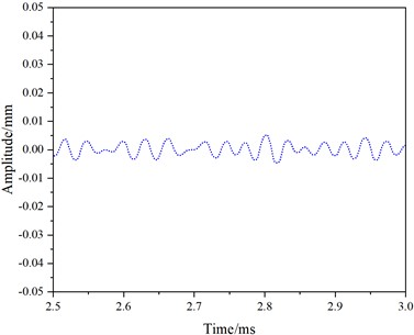
f) 2.5-3.0 ms
Fig. 9 shows the received and reflected waveforms for mode 1 at a frequency of 50 kHz. The first waveform corresponds to the direct wave (Fig. 9(a)), followed by no reflected wave (Fig. 9(c)), and the third waveform represents the reflected wave from the rail end (Fig. 9(e)). The distance between the end face and the receiving position is d=3.45 m. The peak time of the direct wave is t0=0.0673 ms. The peak time of the end face echo is t2=2.3251 ms.
The calculated group velocity for mode 7 at a frequency of 60 kHz using Eq. (12) is V=3138.6 m/s, which differs by only 15.6 m/s from the theoretical group velocity of 3154.2 m/s. This error is within an acceptable range. Therefore, the excited mode is indeed mode 7. Based on the received crack echo signal, the crack position is calculated using Eq. (13), where G represents the theoretical group velocity of the mode:
The simulated calculation result for the crack position is 1.72 m on the rail, which differs by only 0.02 m from the actual crack position of 1.75 m. Therefore, it can be concluded that mode 7 is capable of detecting the transverse crack on the railhead. Similarly, the simulated group velocities and detected crack positions for mode 7 at 40 kHz and mode 1 at 50 kHz are calculated, and the results are shown in Table 4.
Table 4Simulated group velocities and crack positions
Frequency (KHz) | Modal number | Vmg_t (m/s) | Vmg (m/s) | Group velocity error | Crack location | Crack position error | Amplitude of crack echo signal |
6 | 7 | 3138.6 | 3154.3 | 15.6 | 1.72 | 0.02 | 0.00713 |
4 | 7 | 3094.4 | 3112.2 | 17.8 | 1.65 | 0.1 | 0.00451 |
5 | 1 | 3057.8 | 3049.9 | 7.9 | ※ | ※ | 0 |
Note: ※ indicates undetected | |||||||
From the analysis in Table 4, it is evident that the excitation method can successfully induce the 7th mode and the 1st mode. In Fig. 6, the received signal of the 7th mode at 40 kHz has a crack echo, indicating the detection of the lateral crack on the railhead with an error of 0.1 m. However, the amplitude of the crack echo is 36.74 % lower than that of the 7th mode at 60 kHz. In Fig. 7, the received signal of the 1st mode at 50 kHz does not have a crack echo, indicating that the 1st mode cannot detect the lateral crack on the railhead. Therefore, among the three modes, the 7th mode at 60 kHz is the most affected by the lateral crack on the railhead, resulting in the best crack detection performance. Following this, the 7th mode at 40 kHz, with a relatively large crack area energy evaluation index, is the next effective mode for crack detection. Conversely, the lateral crack has the least effect on the 1st mode at 50 kHz, rendering it unable to detect the lateral crack on the railhead-consistent with the calculated results of crack influence on guided wave modes.
Fig. 9Simulation results for mode 1 at a frequency of 50 kHz
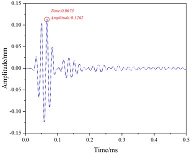
a) 0-0.5 ms
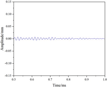
b) 0.5-1.0 ms
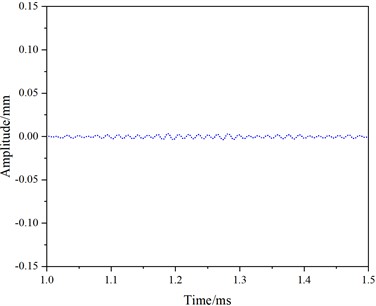
c) 1.0-1.5 ms
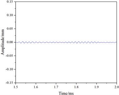
d) 1.5-2.0 ms
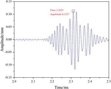
e) 2.0-2.5 ms
f) 2.5-3.0 ms
3.2. Experimental validation
A crack is created on the side of the rail head, as shown in Fig. 10(a), with a rail length of 3.5 m and the crack located at 1.685 m. Excitation is applied to the 7th mode at 60 kHz and the 1st mode at 50 kHz in the rail to verify the analysis results of the crack’s effect on guided wave modes. To excite the 7th mode, two transducers with a center frequency of 60 kHz are vertically attached to nodes 81 and 89 of the rail head at one end of the rail. They are oriented in the same direction and positioned 0.05 m from the end face, with receiving transducers installed nearby. The excitation signal, a 60 kHz sine wave modulated by a five-cycle Hanning window, is generated by a signal generator and applied to the rail via an amplifier. The setup is shown in Figs. 10(b)-(c).
Fig. 10Rail head crack and experimental setup
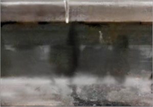
a) Rail head crack
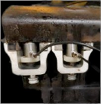
b) Mode 7
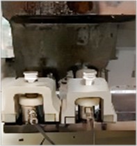
c) Mode 7
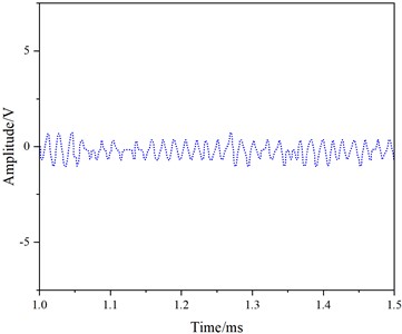
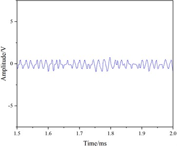
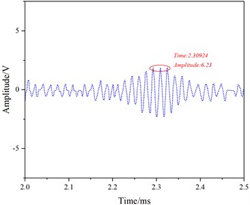
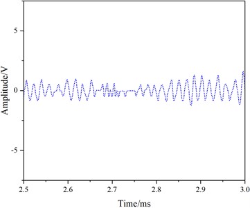
Cracks were intentionally created on the side of the railhead, with a rail length of 3.5 meters and the crack positioned at 1.685 meters. Excitation experiments were conducted in the rail using the 7th mode with a frequency of 60 kHz and the 1st mode with a frequency of 50 kHz to validate the mechanism of crack interaction with guided wave modes, as analyzed theoretically. To stimulate the 7th mode, two transducers with a central frequency of 60 kHz were vertically attached at nodes 81 and 89 on one end of the railhead. They were excited in the same direction, and a receiving transducer was placed 0.05 meters from the end face. The excitation signal, a 60 kHz sinusoidal wave modulated with a Hanning window for five cycles, was generated by a signal generator and applied to the rail through an amplifier. The crack detection experiment for the 7th mode was conducted in 10 sets, and the received signals were collected using an oscilloscope. The results, after averaging processing, are presented in Fig. 11.
In Fig. 11, distinct crack reflection echoes (Fig.11(c)) and end-face reflection signals (Fig. 11(e)) are observable. By calculating the time difference between the crack reflection signal and the direct wave signal peak values, along with extracting the theoretical group velocity of the 7th mode from Tables 3-4, the crack distance from the receiving transducer was computed using Eq. (13) as 1.708 m. The result is only 0.023 m different from the actual distance of 1.685 m. Thus, this mode can effectively detect cracks on the rail head, aligning with the simulated results.
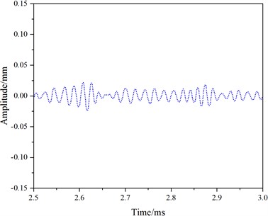
For the excitation of the 1st mode, transducers with a center frequency of 50 kHz were attached at node 11 on one end of the rail. A receiving transducer was installed at node 11 at a distance of 0.05 m. The signal generator provided an excitation signal, a 5-cycle Hanning window-modulated sinusoidal wave at a frequency of 50 kHz. Similarly, 10 sets of received signals were collected and averaged, with results depicted in Fig.12.
From Fig. 12, it is evident that the waveform only contains an end-face reflection signal (Fig. 12(e)), with no crack reflection signal. Consequently, the influence of cracks on the 1st mode is minimal, and the 1st mode cannot detect rail head cracks, aligning with the simulation results.
The comprehensive analysis of simulation and experimental validation leads to the conclusion that the modal crack area energy evaluation index plays a predominant role in the impact of cracks on modes, serving a decisive function. Meanwhile, the modal crack reflection intensity evaluation index plays a secondary role, functioning as a filtering mechanism. In practical applications, the procedure involves calculating the Sre evaluation index first, selecting the corresponding Sre∈[0.95,1] modes, and then calculating their Sri evaluation indices. Modes with higher Sri values are filtered out as the detection modes for the crack. Through simulation and experimental analysis, it is affirmed that the proposed method for optimal mode selection in rail defect detection, based on the sensitivity of guided wave modal cracks, is effective.
Fig. 11Experimental results of 7th Mode at 60 kHz
a) 0-0.5 ms
b) 0.5-1.0 ms
c) 1.0-1.5 ms
d) 1.5-2.0 ms
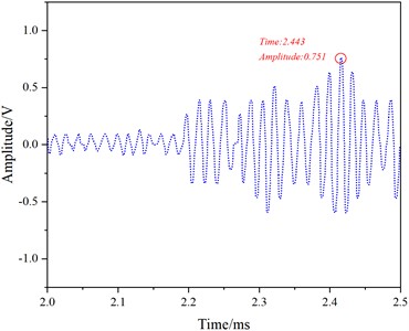
e) 2.0-2.5 ms
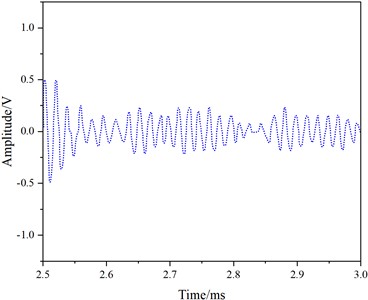
f) 2.5-3.0 ms
Fig. 12Experimental results for the 1st Mode at 50 kHz
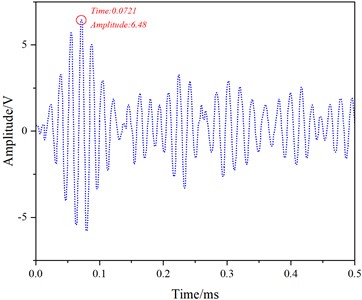
a) 0-0.5 ms
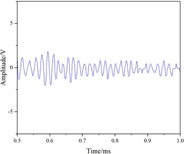
b) 0.5-1. 0 ms
c) 1.0-1.5 ms
d) 1.5-2.0 ms
e) 2.0-2.5 ms
f) 2.5-3.0 ms
4. Conclusions
To achieve the optimal selection of detection modes for different cracks, this paper proposes a method based on the crack sensitivity of guided wave modes. After analyzing the dispersion characteristics and mode properties of guided wave modes, the study establishes evaluation criteria for crack area energy and crack reflection intensity based on the location and trend of crack formation. The mechanism of how cracks affect guided wave modes is studied, enabling the selection of the optimal detection modes for cracks in the rail head region. Simulation and experimental results demonstrate that the guided wave modes selected using this method can accurately identify rail cracks, laying a foundation for further research on rail crack detection and localization methods.
References
-
D. Perfetto, C. Pezzella, V. Fierro, N. Rezazadeh, A. Polverino, and G. Lamanna, “FE modelling techniques for the simulation of guided waves in plates with variable thickness,” Procedia Structural Integrity, Vol. 52, pp. 418–423, Jan. 2024, https://doi.org/10.1016/j.prostr.2023.12.042
-
A. Antonio, N. Rezazadeh, A. Polverino, and S. Beneduce, “Numerical study of ultrasonic guided wave in composite reinforced panels with different stiffener shapes,” Macromolecular Symposia, Vol. 411, p. 23000, 2023.
-
D. Perfetto, N. Rezazadeh, A. Aversano, A. de Luca, and G. Lamanna, “Composite panel damage classification based on guided waves and machine learning: an experimental approach,” Applied Sciences, Vol. 13, No. 18, p. 10017, Sep. 2023, https://doi.org/10.3390/app131810017
-
Q. Li, “New sparse regularization approach for extracting transient impulses from fault vibration signal of rotating machinery,” Mechanical Systems and Signal Processing, Vol. 209, p. 111101, Mar. 2024, https://doi.org/10.1016/j.ymssp.2023.111101
-
C. Zhang, X. Ma, and Q. Bi, “Complex mixed-mode oscillations based on a modified Rayleigh-Duffing oscillator driven by low-frequency excitations,” Chaos, Solitons and Fractals, Vol. 160, p. 112184, Jul. 2022, https://doi.org/10.1016/j.chaos.2022.112184
-
H. Zhao, X. Ma, B. Zhang, and Q. Bi, “Bursting dynamics and the bifurcation mechanism of a modified Rayleigh-van der Pol-Duffing oscillator,” Physica Scripta, Vol. 97, No. 10, p. 105208, Oct. 2022, https://doi.org/10.1088/1402-4896/ac93c0
-
J. Giné and C. Valls, “Liouvillian integrability of a general Rayleigh-Duffing oscillator,” Journal of Nonlinear Mathematical Physics, Vol. 26, No. 2, p. 169, Jan. 2021, https://doi.org/10.1080/14029251.2019.1591710
-
V. Ramanan, A. Ramankutty, S. Sreedeep, and S. R. Chakravarthy, “Dynamical states of thermo-acoustic system with respect to frequency-phase relationship based on probabilistic oscillator model,” Nonlinear Dynamics, Vol. 110, No. 2, pp. 1633–1649, Jul. 2022, https://doi.org/10.1007/s11071-022-07693-z
-
X. Ling, W.-B. Ju, N. Guo, C.-Y. Wu, and X.-M. Xu, “Explosive synchronization in network of mobile oscillators,” Physics Letters A, Vol. 384, No. 35, p. 126881, Dec. 2020, https://doi.org/10.1016/j.physleta.2020.126881
-
R. Al Mahmud, M. O. Faruque, and R. H. Sagor, “A highly sensitive plasmonic refractive index sensor based on triangular resonator,” Optics Communications, Vol. 483, p. 126634, Mar. 2021, https://doi.org/10.1016/j.optcom.2020.126634
-
N. A. Kudryashov, “The generalized Duffing oscillator,” Communications in Nonlinear Science and Numerical Simulation, Vol. 93, p. 105526, Feb. 2021, https://doi.org/10.1016/j.cnsns.2020.105526
-
S. Panahi, F. Nazarimehr, S. Jafari, J. C. Sprott, M. Perc, and R. Repnik, “Optimal synchronization of circulant and non-circulant oscillators,” Applied Mathematics and Computation, Vol. 394, p. 125830, Apr. 2021, https://doi.org/10.1016/j.amc.2020.125830
-
B. Yang, C. Hu, F. Xuan, C. Luo, Y. Xiang, and B. Xiao, “Health monitoring of pressure vessels based on ultrasonic guided waves i: wave propagation behavior and damage localization,” Journal of Mechanical Engineering, Vol. 56, No. 4, pp. 1–10, 2020.
-
B. Xing, Z. Yu, X. Xu, L. Zhu, and H. Shi, “Research on a rail defect location method based on a single mode extraction algorithm,” Applied Sciences, Vol. 9, No. 6, p. 1107, Mar. 2019, https://doi.org/10.3390/app9061107
-
C. M. Lee, J. L. Rose, and Y. Cho, “A guided wave approach to defect detection under shelling in rail,” NDT and E International, Vol. 42, No. 3, pp. 174–180, Apr. 2009, https://doi.org/10.1016/j.ndteint.2008.09.013
About this article

This work is supported by Natural Science Foundation of Guangdong Province (No. 2022A1515011409); supported by Key Areas Special Project of General Universities in Guangdong Province (No. 2023ZDZX1024);supported in part by research grants from the Youth Project of National Natural Science Foundation of China (No. 52105268); supported in part by Shaoguan University Ph.D. Initiation Project (440-9900064604); supported by Shao guan Social Development Science and Technology Collaborative Innovation System Construction Project (No. 230330178036242).
The datasets generated during and/or analyzed during the current study are available from the corresponding author on reasonable request.
Jianjun Liu: conceptualization, formal analysis, supervision, validation, writing-review and editing. Lanlan Fan: investigation, methodology, software, visualization. Huan Luo: resources, writing-original. Senquan Yang: project administration, draft preparation.
The authors declare that they have no conflict of interest.
