Fault diagnosis algorithm based on GADF-DFT and multi-kernel domain coordinated adaptive network

Yin, Caiming; Jiang, Shan; Wang, Wenrui; Jin, Jiangshan; Wang, Zhenming; Wu, Bo

doi:10.21595/jve.2024.23972

Journal of Vibroengineering

Browse Journal

Submit article

Published: 20 July 2024

Check for updates

Fault diagnosis algorithm based on GADF-DFT and multi-kernel domain coordinated adaptive network

Caiming Yin¹

Shan Jiang²

Wenrui Wang³

Jiangshan Jin⁴

Zhenming Wang⁵

Bo Wu⁶

¹University of Chinese Academy of Sciences, Beijing, China

^{1, 2, 3, 5, 6}Shanghai Advanced Research Institute, Chinese Academy of Sciences, Shanghai, China

⁴Shanghai Marine Diesel Engine Research Institute, Shanghai, China

Corresponding Author:

Bo Wu

Cite the article Download PDF

Article in Press

Downloads 10

Abstract

To address the problems of low detection accuracy of rolling bearings under different loads and the difficulty of effectively identifying the lack of labelled data, a rolling bearing fault diagnosis method combining GADF-DFT image coding and Multi-kernel domain coordinated adaptation network is proposed. Firstly, the vibration signal is converted into a two-dimensional image using GADF coding technology, and then the GADF image is converted into the frequency domain using discrete Fourier transform to extract deeper feature information. Combined with the multi-source domain adaptive method, the public feature extraction module is used to initially achieve feature mining of the image; the MK-MMD algorithm of the domain-specific adaptive module reduces the difference in feature distribution between the source and target domains; and the final classification difference minimization module reduces the problems caused by the classification errors that may be generated by the different domain classifiers due to the fact that the data samples are located near the category boundaries. The test uses the Case Western Reserve University dataset and divides the dataset with different operating conditions as the source and target domains, and the test results show that the proposed model demonstrates its effectiveness in responding to the complex operating condition changes in rolling bearing fault detection in multiple operating condition migration tasks, good adaptability and robustness, and is able to achieve accurate fault diagnosis under different operating conditions.

1. Introduction

Rolling bearings are crucial in minimizing friction between shafts in rotating machinery; however, they are susceptible to failure under strenuous operating conditions [1]. The operational normalcy of these bearings is essential for the stable functioning of mechanical equipment, underscoring the necessity of prompt and efficient monitoring and diagnosis of their operational condition [2].

Traditionally, fault diagnosis techniques are categorized into signal processing [3] and data-driven methodologies [4]. Signal processing approaches, including wavelet decomposition [5], empirical modal decomposition [6], and variational modal decomposition [7], principally involve the extraction of fault characteristics by analyzing vibration signals across time, frequency, and time-frequency domains. While effective, these methods demand a considerable depth of expertise and experience for their implementation. In contrast, recent technological advancements have paved the way for data-driven methods, grounded in machine learning and deep learning, to supersede traditional signal processing techniques. Machine learning applications in fault diagnosis, such as support vector machines [8] and random forests [9], exhibit efficacy in fault identification. However, these approaches encounter two primary limitations: firstly, they rely heavily on feature vectors derived from signal processing for input, where the quality of feature extraction significantly influences fault classification outcomes [10]; secondly, given that machine learning requires extensive labeled data for the supervised learning of fault characteristics, it faces challenges in industrial environments where unlabelled data is prevalent [11]. The evolution of computer vision and computational capabilities has notably advanced deep learning algorithms, particularly convolutional and residual neural networks, in machinery fault diagnosis. These advancements facilitate comprehensive, end-to-end intelligent diagnostics of rotating machinery.

In the realm of real-world industrial settings, the task of diagnosing faults in bearings is met with numerous challenges, primarily due to the diverse nature of operational conditions. A primary concern is the variability in the distribution of bearing fault data, which can be attributed to differences in motor load torque. This variability complicates the provision of accurate data labels across a spectrum of operational scenarios, consequently impacting the quality and volume of available samples. Such a scenario hampers the ability to fulfill the data requisites essential for the training of deep learning models [12]. Furthermore, when deep learning models, which are initially trained on a limited set of domain-specific data, are employed in unfamiliar or varying contexts, there is a notable decline in their diagnostic efficacy [13]. Another significant issue is the direct incorporation of one-dimensional signals into network models. This approach may not effectively harness the inherent correlations within the data, thereby amplifying the uncertainty and intricacy involved in diagnosing bearing faults. Given these challenges, exploring novel data processing methodologies that enable precise fault diagnosis on partially labeled data emerges as a crucial area of research.

In light of significant advancements in image recognition and classification [14], the conversion of one-dimensional vibration signals into two-dimensional images has emerged as a promising approach for bearing fault diagnosis. This method leverages the strengths of deep convolutional neural networks in extracting features from two-dimensional imagery. Such a conversion essentially reframes the fault diagnosis of one-dimensional time-series signals as an image classification task. For instance, Cheng Jie [15] et al. successfully automated bearing fault diagnosis by transforming vibration signals into recurrence plots (RP) for subsequent pattern recognition by classifiers. Similarly, Tong Yu [16] et al. employed Gramian Angular Difference Fields (GADF) to encode vibration signals. This encoding facilitated the identification of temporal correlations and the generation of feature maps for input into convolutional neural networks, thereby enabling adaptive fault feature extraction and classification for rolling bearings. However, these methods are not without limitations. The creation of time-frequency diagrams from vibration signals hinges on expert judgment, with parameter selection critically impacting the comprehensive representation of signal information in the resultant images. Additionally, images typically comprise various components-periodic, non-periodic, and noise-intertwined within the spatial domain, complicating direct analysis and separation. While the spatial domain offers insights into the visual aspects of images, it does not readily yield deeper feature information. Furthermore, the effectiveness of conventional deep learning techniques varies when diagnosing rolling bearing defects of different sizes, composite defects, and under variable speed conditions. Consequently, while the approach of converting vibration signals into two-dimensional images within a deep learning framework shows promise, addressing these challenges remains essential to enhance the diagnostic accuracy and applicability.

Deep learning methods typically need to satisfy two conditions to achieve high accuracy [18]: first, the data in the training and test sets must be identically distributed; second, sufficient data annotation is required. However, in real industrial scenarios, these two conditions are often difficult to satisfy simultaneously. Due to the diversity of working environments, there are significant differences in the vibration data distribution of bearings, making it difficult to apply traditional deep learning methods. At the same time, since the bearings are in a healthy state most of the time, with few faults occurring, it is difficult to collect enough fault data and corresponding labels, which further restricts the application of traditional deep learning methods in complex working conditions. To overcome the limitations of traditional deep learning methods, the research of migration learning in the field of fault diagnosis has been deepened [19], especially domain adaptive, which focuses on learning and bridging the differences between the source and target domains, mainly using the annotated data in the source domain to train a generalised fault diagnosis model applicable to the samples in the target domain. It adapts the model trained on the source domain to the task in the target domain by mapping the source and target domain samples to a shared feature space, minimizing the difference in feature distribution between them, and mining their similar features. In addition, in the absence of labeled data in the target domain, the unsupervised domain adaptive approach without labels can effectively use the knowledge of the source domain to enhance the learning capability of the target domain. This approach solves the challenge of insufficient labeled information in the target domain by migrating existing knowledge.

Contemporary research in domain adaptation primarily addresses single-source unsupervised domain adaptation challenges. While single-source domain adaptation methods are effective in scenarios where data distribution is largely consistent, they may fall short in complex working environments. In such settings, the data and insights gleaned from a single source may not adequately represent the target domain's diversity and complexity [20]. This limitation becomes evident when these methods struggle to generalize effectively to target domains that significantly differ from the source domain. On the other hand, multi-source domain adaptation offers a robust alternative. By amalgamating data and knowledge from various source domains, multi-source methods provide a richer and more varied pool of information. Each source domain contributes unique insights reflecting different conditions and characteristics, thereby enabling a more nuanced understanding of the target domain’s complexity. Consequently, multi-source domain adaptation is particularly adept at navigating complex and variable work conditions, proving especially beneficial when bridging substantial disparities between source and target domains.

Based on the above research foundation, this paper proposes a multi-source domain adaptive migration learning model based on Multi-Kernel Domain Coordinated Adaptation Network (MKDCAN) based on GADF-DFT. First, the one-dimensional vibration signal is converted into a two-dimensional image by the GADF algorithm, which has a unique mapping relationship with the time series before the conversion. Then, the Discrete Fourier Transform (DFT) is used and the deep feature information in the image can be mined more deeply by frequency domain analysis. Finally, after processing and transforming the image data, these data are used as source domain inputs to achieve accurate fault diagnosis by integrating diagnostic knowledge from multiple source domains using MKDCAN.

2. GADF-DFT

2.1. Gramian angular field

Gram angle field coding is an image coding technique that converts a one-dimensional time-series signal into a two-dimensional image by means of a dimensional transformation of the Gram matrix data in polar coordinates. GADF coding is particularly suitable for the analysis of vibration signals due to its ability to efficiently measure correlations between points in the signal over time by means of a trigonometric transformation of the angular difference, and by transforming the image texture to visualization of these correlations by transforming the image texture, preserving the full information of the vibration signal as well as enhancing the identification of faults in the signal [21].

First, the collected data set $X$ is partitioned into $n$ collection points based on the collection frequency of the vibration signal, i.e. $X = \{x_{1}, x_{2}, \dots, x_{n}\}$ , where the deflation process is performed on $X$ to normalise all data in $X$ to between [–1, 1], where $1 \leq i \leq n$ :

1

\tilde{X} = \frac{[x_{i} - m a x (X)] + [x_{i} - m i n (X)]}{m a x (X) - m i n (X)} .

Fig. 1GADF image encoding process

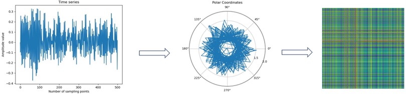
The deflated value $\tilde{X}$ is then encoded as the angular cosine α and the time node $t_{i}$ is encoded as the radius $R$ . $R$ is the distance from the locus of the polar coordinate system to the origin of the polar coordinates:

2

\{\begin{array}{l} α = \arccos ({\tilde{x}}_{i}), - 1 \leq {\tilde{x}}_{i} \leq 1, {\tilde{x}}_{i} \in \tilde{X}, \\ R = \frac{t_{i}}{N}, t_{i} \in N . \end{array}

In the above equation, the unit length of the polar coordinate system is divided equally into equal parts, and in Eq. (2) the angle $α$ in polar coordinates corresponds to the data points in the time series, and this correspondence preserves the temporal information of the vibration signal. In this way, the radius in polar coordinates can be used to determine the time value of each point in the time series.

Finally, by applying the trigonometric difference angle formula between each point, it is possible to reflect the temporal correlation of each point at different time intervals. This method uses changes in angle to quantify the relationship between different time points in a time series, thus revealing the temporal structure and dynamic properties within the signal:

3

G = [\begin{matrix} s i n (α_{1} - α_{1}) & \dots & s i n (α_{1} - α_{n}) \\ ⋮ & ⋮ \\ s i n (α_{n} - α_{1}) & \dots & s i n (α_{n} - α_{n}) \end{matrix}] = \sqrt{I - {({\tilde{X}}^{2})}^{T}} \cdot \tilde{X} - {\tilde{X}}^{T} \cdot \sqrt{I - {\tilde{X}}^{2}} .

The above transformation transforms the time series into a two-dimensional feature image that is symmetric along the diagonal. In order to create a symmetric two-dimensional feature image and retain the temporal features within the time series, the specific implementation process is shown in Fig. 1.

2.2. Discrete Fourier transform of images

A one-dimensional signal is essentially a combination of several sinusoids of different frequencies, and the Fourier transform is the conversion of these signals from the time domain to the frequency domain, a process reflected in the following equation:

4

F (ω) = \int_{- \infty}^{+ \infty} f (t) e^{- i ω t} d t .

A two-dimensional signal can be regarded as the superposition of multi-frequency sinusoidal plane waves, and a two-dimensional image is essentially composed of a discrete and finite number of pixel points, so the two-dimensional Fourier transform of the image must be applied in a discrete manner, and the transform equation is shown in Eq. (5):

5

F (μ, v) = \sum_{x = 0}^{M - 1} \sum_{y = 0}^{N - 1} f (x, y) e^{- j 2 π (\frac{μ x}{M} + \frac{v y}{N})},

where $f (x, y)$ is the pixel value of $(x, y)$ in the spatial domain coordinates of the image, $F (μ, v)$ is the spectrum of the image in the frequency domain, $M$ and $N$ are the dimensions of the image.

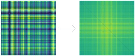
Images contain periodic components, non-periodic components and noise, and it is difficult to analyze and separate these components directly from the spatial domain. Converting an image from the spatial domain to the frequency domain for analysis provides a different perspective for understanding and analyzing the image content; in the frequency domain, the image is represented as a collection of components with different frequencies, making it easier to distinguish and extract different features in the image.

3. MKDCAN

The migration learning framework of Multi-Kernel Domain Harmoniser and Adaptation Network (MKDCAN) model takes advantage of the deep neural network model with the advantage of mining the deep features of the data, and adopts the deep neural network model for migration learning feature extraction for multi-source domain fault diagnosis. In turn, a mechanical fault diagnosis method based on multi-source domain deep migration learning is proposed, and its fault diagnosis model is shown in Fig. 2. The fault diagnosis model of MKDCAN mainly consists of three parts: the public feature extraction module, the domain-specific adaptive module, and the classification difference minimisation module.

Fig. 2The structure of MKDCAN

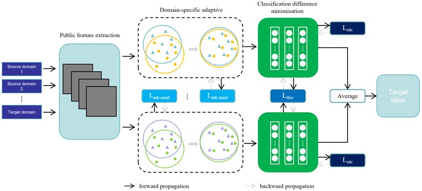
3.1. Public feature extraction module

In the public feature extraction part, a public subnetwork is used to extract the public representation of all the domains that map the 2D image from the original feature space to the public feature space. The public feature extraction module uses the ResNet18 network, and to ensure that the model can extract as many fusion features as possible under different operating conditions, the network shares weights and biases, thus reducing the computational cost. The specific parameters are shown in Table 1.

Table 1The structure of public feature extraction module

Module	Layer	Output shape
ResNet	Input layer	3×224×224
	Conv2d-BN-ReLU	64×112×112
	MaxPool2d	64×56×56
	Sequential	64×56×56
	Sequential	128×28×28
	Sequential	256×14×14
	Sequential	512×7×7
AddNet	Conv2d-BN-ReLU	256×7×7
	Conv2d-BN-ReLU	256×7×7
	Conv2d-BN-ReLU	256×7×7
	AvgPool2d	256×1×1
	Output layer	10

3.2. Domain-specific adaptive module

The domain-specific adaptive module is designed to ensure that each pair of source and target domain data is mapped to a specific feature space. Given a batch image $x_{2}$ from source domain $(X_{s j}, Y_{s j})$ and $X_{s j}$ batch image $X_{t}$ from target domain, the domain-specific adaptive module receives the public features $F (X_{s j})$ and $F (X_{t})$ from the public feature extraction module. $N$ non-shared subnetworks of domain-specific features are then extracted for each source domain $(X_{s j}, Y_{s j})$ , mapping each pair of source and target domains to a specific feature space. The main goal of domain-specific adaptation is to learn domain-invariant feature representations that reduce the differences in feature distributions across domains by using different distance metrics, common metrics are Maximum Mean Discrepancy (MMD) loss [22], Correlation Alignment (CORAL) [23], Multi-Kernel Maximum Mean Discrepancy (MK-MMD) loss [24] and so on.

MK-MMD is a method for measuring the difference between two probability distributions based on the principle of using a set of kernel functions to compute the mean difference between two data distributions. Compared to MMD, which use only a single kernel for transformation, MK-MMD enhances its effect by linearly combining multiple kernels to obtain an optimal kernel. This multi-kernel approach is able to combine the strengths of different kernels to capture and reflect the effects of MMD in a more comprehensive way, making it more effective when dealing with complex data distributions. The MK-MMD method is chosen for the domain-specific adaptive module to measure the distributional differences between domains with the following formula:

6

M K - M M D^{2} (X_{s j}, X_{t}) = {∥\frac{1}{m} \sum_{i = 1}^{m} ϕ_{k} (x_{i}^{s_{j}}) - \frac{1}{n} \sum_{j = 1}^{n} ϕ_{k} (x_{j}^{t})∥}_{H_{k}}^{2},

where $ϕ_{k}$ is the feature mapping to the regenerated kernel Hilbert space $H_{k}$ with kernel $k$ , $m$ and $n$ are the number of samples in the source domain $X_{s j}$ and the target domain $X_{t}$ .

3.3. Classification difference minimization module

The classification difference minimization module uses a softmax classifier $C$ , which is a multi-output network of $N$ domain-specific predictors ${\{C_{j}\}}_{j = 1}^{N}$ , after receiving the domain invariant features processed by the source domain specific domain adaptive module $H (F (x))$ . For each classifier, the classification loss is increased by calculating the cross-entropy, for $N$ source domain knowledge, its cross-entropy classification loss is calculated separately and summed to obtain Eqs. (7):

7

{L o s s}_{s d c} = \sum_{j}^{N} E_{x \sim X_{s j}} J (C_{j} (H_{j} (F (x_{j}^{s_{j}}))), y_{j}^{s_{j}}) .

Furthermore, different domain classifiers may produce classification errors when samples in the target domain are close to category boundaries. This is because each domain-specific classifier is optimized for its source domain, it may not be able to predict accurately when confronted with data in the target domain that has a different distribution from that of the source domain, highlighting the importance of category boundary alignment in both migration learning and domain adaptation tasks. To address this issue, the literature [25] proposes a multi-source fusion classifier to minimize the differences between all classifiers:

8

{L o s s}_{d i s c} = \frac{2}{N \times (N - 1)} \sum_{j = 1}^{N - 1} \sum_{i = j + 1}^{N} E_{x \sim X_{t}} (|C_{i} (H_{i} (F (x_{k}))) - C_{j} (H_{j} (F (x_{k})))|) .

In summary, the total loss term of the MKDCAN model is made up of 3 components, which are denoted as follows:

9

L o s s = {L o s s}_{s d c} + λ {L o s s}_{m k - m m d} + γ {L o s s}_{d i s c},

where $λ$ and $γ$ are the weights of ${L o s s}_{m k - m m d}$ and ${L o s s}_{d i s c}$ respectively, and the model is mainly trained using the standard stochastic gradient descent (SGD) algorithm. In order to reduce the effect of noise at the beginning of training, a strategy of gradual adaptation is used instead of keeping the adaptation factors $λ$ and $γ$ constant. By gradually increasing $λ$ and $γ$ from 0 to 1, tuning is performed according to the formula $λ = γ = \frac{2}{e x p (- θ p)} - 1$ , which remains fixed throughout the experiment [26]. This gradual tuning approach significantly improves the parameter stability of MKDCAN and also simplifies the model selection process.

4. Bearing fault diagnosis based on GADF-DFT and MKDCAN

The specific steps of the bearing fault diagnosis method based on GADF-DFT and MKDCAN are as follows:

1. The acquired signal is converted to a GADF image, and the GADF image is discrete Fourier transformed. Fig. 3 shows the specific conversion.

2. The transformed image is divided into source and destination areas according to different working conditions.

3. For each iteration $t$ , where $t$ goes from 1 to $T$ , set the number of training iterations $T$ :

a. Take a random sample of $m$ images from one of the $N$ source domains, denoted as ${\{x_{s_{j}}^{i}, y_{s_{j}}^{i}\}}_{i = 1}^{m}$ .

b. Take a sample of $m$ images from the target domain, denoted as ${\{x_{t}^{i}\}}_{i = 1}^{m}$ .

c. The source domain samples and target domain samples are input to the public feature extraction module to obtain the common potential representations $F (x_{s_{j}}^{i})$ and $F (x_{t}^{i})$ .

d. The common potential representations of the source samples are input into the domain-specific adaptive module to obtain the domain-specific representation $H_{j} (F (x_{s_{j}}^{i}))$ of the source samples.

e. Feed the domain-specific representations of the source samples into the domain-specific classification module to obtain $C_{j} (H_{j} (F (x_{s_{j}}^{i})))$ and classify them.

f. Feed the common latent representations of the target samples into all domain-specific adaptive modules to obtain domain-specific representations of the target samples $H_{1} (F (x_{t 1}^{i})), \dots, H_{N} (F (x_{t N}^{i}))$ .

g. The MK-MMD loss is calculated using $H_{j} (F (x_{s_{j}}^{i}))$ and $H_{j} (F (x_{t 1}^{i}))$ . Use $H_{1} (F (x_{t 1}^{i})), \dots, H_{N} (F (x_{t N}^{i}))$ to calculate the loss of differences between classification modules.

h. Update the public feature extractor $F$ , several domain specific adaptive modules $H_{1}, \dots, H_{N}$ and several classification modules $C_{1}, \dots, C_{N}$ to obtain the total loss.

Fig. 3Converting GADF images to GADF-DFT images

5. Experiment

5.1. Dataset introduction

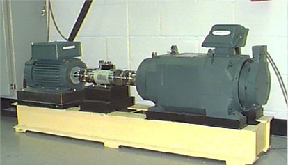
The data set used for the experiment is the bearing failure data set from Case Western Reserve University (CWRU). The experimental data were collected by accelerometers mounted on the drive end and fan end of the motor, the bearing type used on the drive end was 6205-2RS JEM SKF deep groove ball bearings, the bearing type used on the fan end was 6203-2RS JEM SKF deep groove ball bearings, and the rotational speeds of the motor included 1730, 1750, 1772, 1797 r/min, the corresponding motor load is 0, 1, 2, 3hp (1 hp = 0. 746 kW), the sampling frequency includes 12 kHz and 48 kHz, the data used in this section of the experiment is the data at 12 kHz sampling frequency, the sampling time is 10s, the test equipment is shown in Fig. 4.

Fig. 4CWRU bearing data acquisition device

In the CWRU dataset, the bearing failure diameters selected in this paper are 0.1778, 0.3556 and 0.5334 mm, respectively, and the CWRU dataset includes the failure types of inner race fault, outer race fault and rolling ball fault, as well as the normal condition data, which is 10 types in total. The whole dataset is divided into training dataset and test dataset, which are shown in Table 2. Each image comprises 512 sample points, representing the length of each vibration signal segmentation interval. This ensures that 300 samples are constructed for each type of signal feature, with all samples labelled using one-hot coding to distinguish between ten different bearing operating states. Furthermore, the dataset is divided in a ratio of 70 % training set and 30 % testing set, which ensures the availability of a standardised and high-quality database for the training and testing of the deep learning model.

Table 2Classification of bearing fault

Label	Bearing states	Fault diameter / mm	Sample length
0	Rolling ball fault	0.1778	512
1	Rolling ball fault	0.3556	512
2	Rolling ball fault	05334	512
3	Inner race fault	0.1778	512
4	Inner race fault	0.3556	512
5	Inner race fault	05334	512
6	Normal	*	512
7	Outer race fault	0.1778	512
8	Outer race fault	0.3556	512
9	Outer race fault	05334	512

5.2. Feasibility experiment on image coding

In order to evaluate the effectiveness and performance of the GADF-DFT image coding technique in rolling bearing fault detection, several experimental methods are designed for comparative analysis in this study. The specific methods are as follows:

1. Using GADF images, the images are fed into the MKDCAN model.

2. Using GADF-DFT images and inputting the images to the MKDCAN model.

3. The vibration signal is converted to Gramian Angular Summation Field (GASF) and input to the MKDCAN model.

4. Perform a Discrete Fourier Transform on the GASF and input the image into the MKDCAN model.

5. Convert the vibration signal to a Recurrence Plot (RP) and input it to the MKDCAN model.

6. Perform a Discrete Fourier Transform on the RP and use the result again as input to the model.

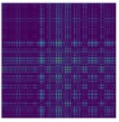
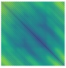
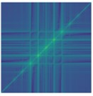
Image coding for different methods as shown in Fig. 5.

Fig. 5Image coding for different methods

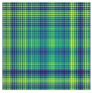
a) GADF

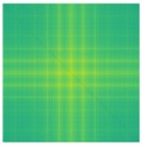
b) GADF-DFT

c) GASF

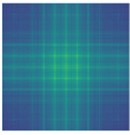
d) GASF-DFT

e) RP

f) RP-DFT

The data used in this experiment is from the CWRU dataset, which is divided into datasets according to different operating conditions and fault types. The resolution of the images generated is 256×256 pixels. For the same experimental scenario, the source and target domain data are input according to the same image coding method.

The accuracy results of the test set are shown in Fig. 6, with the increase of the number of iterations, except for the model with RP-coded images as input, the other models reach convergence at about 10 iterations, and their fault detection accuracy curves all tend to be stable, compared with other coding methods, the model of the RP image coding method fluctuates more, which may be due to the fact that RP image coding works by analyzing the reproducibility of the time series between the different points in time.

GADF and GASF can better capture the overall trend and periodicity characteristics of the data by taking into account the relative angles of the time points in the time series, and GADF and GASF are better able to capture the fundamental modes and frequency components of the vibration signals, whereas RP may emphasize more the dynamic interactions and variations, which may not be the most stable feature to distinguish between different fault types; Furthermore, in multi-source domain adaptation, the model needs to extract and fuse useful information from different source domains and apply it to the target domain, and if the features captured by RP coding vary significantly between source domains or with the target domain, the model may have difficulty in finding a stable domain-invariant representation.

Fig. 6Comparison of different image coding methods

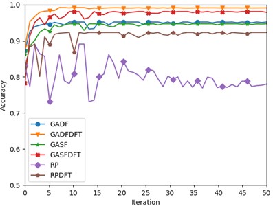
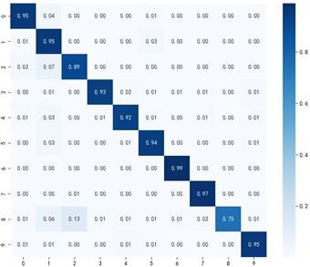
Among the models with other coding methods as input, GADF-DFT image coding has the highest fault diagnosis accuracy, with fault recognition accuracy up to 99.29 %, and the model is more stable. It can be clearly seen from the above data sets that, first of all, compared with GASF coding, GADF coding has a better effect because GADF constructs images by calculating the angle difference between different time points in the time series, which can better reveal the dynamic changes of vibration signals and potential fault characteristics. Secondly, compared with GADF coding, GADF-DFT coding has a better detection effect because the GADF-DFT coding method can effectively distinguish periodic and non-periodic components in images by using two-dimensional discrete Fourier transform conversion from the spatial domain to the frequency domain. This conversion allows us to view images from the perspective of frequency, revealing the details and characteristics that are difficult to identify in the direct spatial representation, and the analysis is carried out in the frequency domain, so that the signal components that were originally mixed in the spatial composite image can be effectively separated, thus strengthening the extraction and recognition of the key features of fault diagnosis. Therefore, through the introduction of frequency domain analysis, GADF-DFT coding not only improves the acquisition of the original signal characteristics, but also improves the ability to distinguish the bearing state.

5.3. Comparison experiment between single-source domain and multi-source domain

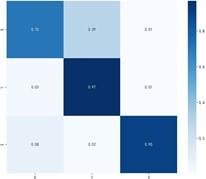
This section will test the four different load conditions of the bearing failure data set, labelled Hp0, Hp1, Hp2 and Hp3 respectively (corresponding to the speed of 1797 rpm, 1772 rpm and 1750 rpm, 1730 rpm). Assume that the multi-source domain task is set to Hp0-Hp1→Hp2, which means that Hp0 and Hp1 are both labelled source domains, Hp2 is unlabeled target domains, and the corresponding single-source domain tasks are set to Hp0→Hp2 and Hp1→Hp2.The comparison schemes and results of the tests in this section are shown in Table 3 and Fig. 7.

This analysis reveals that in transfer learning scenarios encompassing multiple operating conditions, the model's classification accuracy generally surpasses that of migrations from a single source domain to the target domain. More concretely, models trained on data amalgamated from two distinct operating conditions exhibited an increase in classification accuracy by as much as 3.30 percentage points compared to those trained on data from a single condition.

Furthermore, a comparative analysis of the classification accuracy evolution in tasks migrated from a single case versus multiple cases underscores the enhanced performance stability offered by multi-source transfer learning methods. This observation underscores the criticality of integrating data from diverse conditions in multi-source migration learning. It not only contributes to heightened accuracy but also significantly bolsters the stability of the model.

Table 3Basic size and style requirements

Multi-source domain task	Average accuracy	Single-source domain task	Average accuracy	Percentage increase
Hp0-Hp1→Hp2	99.29 %	Hp0→Hp2 Hp1→Hp2	98.28 % 98.67 %	0.10 % 0.06 %
Hp0-Hp1→Hp3	98.34 %	Hp0→Hp3 Hp1→Hp3	97.62 % 97.60 %	0.74 % 0.76 %
Hp0-Hp2→Hp1	99.06 %	Hp0→Hp1 Hp2→Hp1	98.25 % 98.40 %	0.82 % 0.67 %
Hp0-Hp2→Hp3	99.31 %	Hp0→Hp3 Hp2→Hp3	96.14 % 98.77 %	3.30 % 0.55 %
Hp0-Hp3→Hp1	99.40 %	Hp0→Hp1 Hp3→Hp1	98.68 % 97.72 %	0.73 % 1.72 %
Hp0-Hp3→Hp2	99.25 %	Hp0→Hp2 Hp3→Hp2	98.50 % 98.47 %	0.76 % 0.79 %
Hp1-Hp2→Hp0	99.13 %	Hp1→Hp0 Hp2→Hp0	98.76 % 98.35 %	0.37 % 0.79 %
Hp1-Hp2→Hp3	99.34 %	Hp1→Hp3 Hp2→Hp3	97.33 % 98.32 %	2.07 % 1.03 %
Hp1-Hp3→Hp0	98.73 %	Hp1→Hp0 Hp3→Hp0	97.45 % 97.12 %	1.31 % 1.66 %
Hp1-Hp3→Hp2	98.97 %	Hp1→Hp2 Hp3→Hp2	98.91 % 98.12 %	0.06 % 0.86 %
Hp2-Hp3→Hp0	99.32 %	Hp2→Hp0 Hp3→Hp0	98.99 % 98.01 %	0.33 % 1.34 %
Hp2-Hp3→Hp1	99.40 %	Hp2→Hp1 Hp3→Hp1	99.03 % 98.70 %	0.37 % 0.71 %

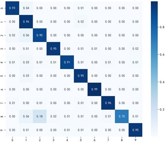
5.4. Comparison of MKDCAN with other multi-source domain methods

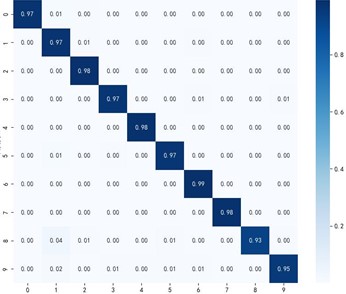
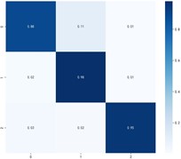
In order to evaluate the performance of the proposed MKDCAN method in mechanical fault diagnosis, the method is compared with several transfer learning algorithms in the current field. The comparison algorithm including joint distribution (JDA), cointegration relationship alignment (CORAL), source domain merging to net adaptation (MSDAN), multi-source vs. net adaptation (MAAN), and domain vs. net adaptation (DANN). By comparing the same 12 types of multi-source domain transfer learning tasks, the accuracy and generalization ability of these methods in different fault diagnosis tasks can be comprehensively evaluated. In particular, the average classification accuracy of the proposed method on various tasks was 99.13 %, which was significantly higher than the average accuracy of the JDAs, CORALs, MSDANs, MAANs and DANNs, which was 89. 03 %, 87.15 %, 91.09 %, 92.32 % and 97.72 %, respectively. This significant performance difference indicates that the proposed method can abstract and exploit cross-domain features more effectively in the face of multi-source domain data, thus improving the accuracy of fault diagnosis and the stability of the model.

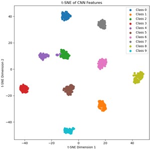
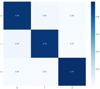
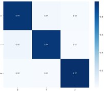
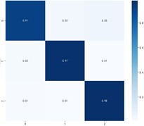
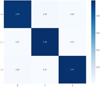
Fig. 8 shows the classification effectiveness of the multi-source domain adaptive algorithm MKDCAN and other multi-source domain adaptive algorithms in the bearing fault diagnosis task. From Figs. 4-3(f), it can be observed that the MKDCAN algorithm proposed in this paper achieves the highest accuracy in fault type diagnosis, effectively reducing the number of misclassified samples. This result demonstrates the superior performance of MKDCAN in dealing with the problem of adaptive fault diagnosis in multi-source domains.

Fig. 7Visualization of single-source and multi-source domain feature distributions

a) Hp0→Hp2

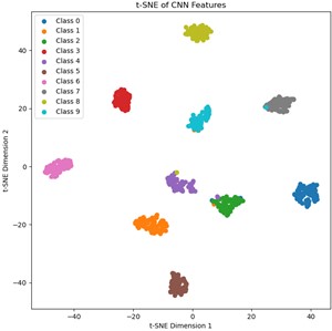
b) Hp1→Hp2

c) Hp0-Hp1→Hp2

Table 4Comparison of MKDCAN with other multi-source domain methods

Multi-source domain task	CORAL	JDA	MSDAN	MAAN	DANN	MKDCAN
Hp0-Hp1→Hp2	90.34 %	93.41 %	92.69 %	89.98 %	96.01 %	99.29 %
Hp0-Hp1→Hp3	87.67 %	87.78 %	90.05 %	91.65 %	97.37 %	98.34 %
Hp0-Hp2→Hp1	88.92 %	92.49 %	93.72 %	94.53 %	98.46 %	99.06 %
Hp0-Hp2→Hp3	89.05 %	89.15 %	91.36 %	93.17 %	98.13 %	99.31 %
Hp0-Hp3→Hp1	83.78 %	87.85 %	90.58 %	91.29 %	98.95 %	99.40 %
Hp0-Hp3→Hp2	82.99 %	85.66 %	88.34 %	90.70 %	99.60 %	99.25 %
Hp1-Hp2→Hp0	88.53 %	91.43 %	93.07 %	95.64 %	98.78 %	99.13 %
Hp1-Hp2→Hp3	87.36 %	85.94 %	89.66 %	90.98 %	97.59 %	99.34 %
Hp1-Hp3→Hp0	87.60 %	89.42 %	90.40 %	92.26 %	97.77 %	98.73 %
Hp1-Hp3→Hp2	88.31 %	88.98 %	90.93 %	92.05 %	97.67 %	98.97 %
Hp2-Hp3→Hp0	84.83 %	86.10 %	89.78 %	91.75 %	95.26 %	99.32 %
Hp2-Hp3→Hp1	86.45 %	90.17 %	92.45 %	93.81 %	97.04 %	99.40 %
Average accuracy	87.15 %	89.03 %	91.09 %	92.32 %	97.72 %	99.13 %

6. Comparative experiments with different datasets

In order to thoroughly verify the generalizability of the MKDCAN model proposed in this paper, fault diagnosis experiments on different datasets are performed in this section. By testing the model on multiple datasets, the performance of MKDCAN can be more comprehensively evaluated to ensure that it can still maintain its efficient and accurate fault diagnosis capability in a variable real-world application environment. In this section, the bearing dataset from the University of Paderborn (PU) is selected to verify the fault diagnosis performance of MKDCAN on different datasets.

Fig. 8Visualization of single-source and multi-source domain feature distributions

a) CORAL

b) JDA

c) MSDAN

d) MAAN

e) DANN

f) MKDCAN

The PU bearing data set is a rolling bearing type 6203, which includes three states of normal operation, inner ring failure and outer ring failure, the sampling frequency of the sample is set to 64 kHz, and 15 sets of bearing data are selected to cover the vibration of bearings under four load conditions, and the data of inner ring failure, outer ring failure and the three states of normal operation have been recorded in each load condition, and the data of the PU data set are shown in Table 5. The actual failure information from the accelerated fatigue test at a running speed of 1500 rpm in this data set was selected for the experiment, and the radial forces F experienced by the bearings were 1000 N and 400 N, and the load torques $M$ were 0.7 N·m and 0.1 N·m. The length of each image in this dataset is set to 500, and the training set and test set are divided according to the ratio of 7:3. The specific classification is shown in Table 6 and the data set is divided into four types of data sets according to different working conditions. For example, the working condition N15_M07_F10 means that the data set is collected at the operating speed of 1500 rpm, the loading torque of 0.7 N·m, and the radial force of the bearing is 1000 N.

Table 5PU rolling bearing dataset

Fault type	IR	OR	Normal
Fault label	0	1	2
Bearing designation	KA04	KI04	K001
	KA15	KI14	K002
	KA16	KI16	K003
	KA22	KI18	K004
	KA30	KI21	K005

Table 6Classification of PU bearing datasets

Fault type		IR	OR	Normal	Working condition
Fault label		0	1	2	Working condition
Ⅰ	Train	700	700	700	N15_M07_F10
Ⅰ	Test	300	300	300	N15_M07_F10
Ⅱ	Train	700	700	700	N15_M01_F10
Ⅱ	Test	300	300	300	N15_M01_F10
Ⅲ	Train	700	700	700	N15_M07_F04
Ⅲ	Test	300	300	300	N15_M07_F04

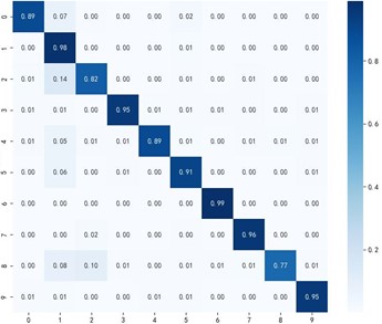
The experimental settings in this section refer to the previous section, and the experimental results are shown in Table 7. As can be seen from the table, the MK-IMFSAN method performs well in all the comparative experiments, with an average fault diagnosis accuracy of 97.36 %, which ranks first among all the comparative methods.

Fig. 9Classification effectiveness of domain adaptive algorithms on the PU dataset

a) CORAL

b) JDA

c) MSDAN

d) MAAN

e) DANN

f) MKDCAN

Fig. 9 shows the specific classification effects of the six domain adaptive methods, and these plots further confirm that MKDCAN performs significantly better than the other algorithms. The experimental results confirm that the MKDCAN algorithm maintains its good recognition accuracy, high generalization and robustness in dealing with multi-source domain adaptive fault diagnosis problems across datasets.

Table 7Experimental results of cross-domain diagnosis under PU dataset

Multi-source domain task	CORAL	JDA	MSDAN	MAAN	DANN	MKDCAN
Ⅰ+Ⅱ→Ⅲ	86.98 %	88.96 %	91.04 %	93.39 %	97.54 %	98.52 %
Ⅰ+Ⅲ→Ⅱ	87.54 %	88.84 %	91.29 %	93.12 %	97.49 %	98.19 %
Ⅱ+Ⅲ→Ⅰ	85.16 %	86.27 %	88.37 %	90.40 %	94.79 %	95.38 %
Average accuracy	86.56 %	88.02 %	90.23 %	92.30 %	96.62 %	97.36 %

7. Conclusions

In this paper, an innovative multi-source domain adaptive migratory learning model, GADF-DFT-based multi-kernel domain coordinated adaptive network is proposed, which converts one-dimensional vibration signals into two-dimensional images and performs deep frequency domain analysis. This method not only overcomes the limitations of traditional deep learning methods under complex working conditions, but also improves the accuracy and applicability of fault diagnosis. The experimental results show that the GADF-DFT image coding method has stronger fault-specific recognition, while compared with other multi-source domain adaptive methods, MKDCAN achieves an average fault diagnosis accuracy of 99.13 % in the case of missing labels, which has better recognition accuracy and robustness. Meanwhile, the experimental results under different datasets show that MKDCAN has better classification effect, which further validates the generalization and robustness of MKDCAN model.

References

B. Yang, J. W. Zhang, J. G. Wang, C. Zhang, and B. Qin., “Extraction of early fault feature of rolling bearing based on MED-RSSD,” Journal of Mechanical Transmission, Vol. 42, No. 6, pp. 120–124, 2018, https://doi.org/10.16578/j.issn.1004.2539.2018.06.025

Publisher
Y. Qin, “A new family of model-based impulsive wavelets and their sparse representation for rolling bearing fault diagnosis,” IEEE Transactions on Industrial Electronics, Vol. 65, No. 3, pp. 2716–2726, Mar. 2018, https://doi.org/10.1109/tie.2017.2736510

Publisher
X. Z. Zhao, B. Y. Ye, and T. J. Chen, “Multi-resolution singular value decomposition and its application in signal processing and fault diagnosis,” Journal of Mechanical Engineering, Vol. 46, No. 20, 2010.

Publisher
X. Lou and K. A. Loparo, “Bearing fault diagnosis based on wavelet transform and fuzzy inference,” Mechanical Systems and Signal Processing, Vol. 18, No. 5, pp. 1077–1095, Sep. 2004, https://doi.org/10.1016/s0888-3270(03)00077-3

Publisher
K. Deák and I. Kocsis, “Support vector machine with wavelet decomposition method for fault diagnosis of tapered roller bearings by modelling manufacturing defects,” Periodica Polytechnica Mechanical Engineering, Vol. 61, No. 4, p. 276, Sep. 2017, https://doi.org/10.3311/ppme.10802

Publisher
R. Abdelkader, A. Kaddour, A. Bendiabdellah, and Z. Derouiche, “Rolling bearing fault diagnosis based on an improved denoising method using the complete ensemble empirical mode decomposition and the optimized thresholding operation,” IEEE Sensors Journal, Vol. 18, No. 17, pp. 7166–7172, Sep. 2018, https://doi.org/10.1109/jsen.2018.2853136

Publisher
T. Zhang, J. Zhang, H. Xue, C. Wang, W. Han, and K. Li, “Prediction of distribution network operation trend based on the secondary modal decomposition and LSTM-MFO algorithm,” in 6th Asia Conference on Power and Electrical Engineering (ACPEE), pp. 520–525, Apr. 2021, https://doi.org/10.1109/acpee51499.2021.9436870

Publisher
C. Gao, Z. Liao, and S. Huang, “Fault diagnosis of commutation failures in the HVDC system based on wavelet singular value and support vector machine,” in Asia-Pacific Power and Energy Engineering Conference, pp. 1–4, Mar. 2009, https://doi.org/10.1109/appeec.2009.4918374

Publisher
Y. Santur, M. Karaköse, and E. Akin, “Random forest based diagnosis approach for rail fault inspection in railways,” in National Conference on Electrical, Electronics and Biomedical Engineering (ELECO), pp. 745–750, 2016.

Search CrossRef
Y. K. Gu, K. Wu, and C. Li., “Rolling bearing fault diagnosis based on Gram angle field and transfer deep residual neural network,” Journal of Vibration and Shock, Vol. 41, No. 21, pp. 228–237, 2022, https://doi.org/10.13465/j.cnki.jvs.2022.21.025

Publisher
J. Shao, Z. Huang, Y. Zhu, J. Zhu, and D. Fang, “Rotating machinery fault diagnosis by deep adversarial transfer learning based on subdomain adaptation,” Advances in Mechanical Engineering, Vol. 13, No. 8, p. 168781402110402, Aug. 2021, https://doi.org/10.1177/16878140211040226

Publisher
D. Peng, Z. Liu, H. Wang, Y. Qin, and L. Jia, “A novel deeper one-dimensional CNN with residual learning for fault diagnosis of wheelset bearings in high-speed trains,” IEEE Access, Vol. 7, pp. 10278–10293, Jan. 2019, https://doi.org/10.1109/access.2018.2888842

Publisher
P. Wei, Y. Li, Z. Zhang, T. Hu, Z. Li, and D. Liu, “An optimization method for intrusion detection classification model based on deep belief network,” IEEE Access, Vol. 7, pp. 87593–87605, Jan. 2019, https://doi.org/10.1109/access.2019.2925828

Publisher
K. Zhang, X. H. Feng, and Y. R. Guo, “Overview of deep convolutional neural network for image classification,” Journal of Image and Graphics, Vol. 26, No. 10, pp. 2305–2325, 2021, https://doi.org/10.11834/jig.200302

Publisher
J. Cheng and S. R. Li, “Bearing fault diagnosis based on recurrence plots and local non-negative matrix factorization,” Industry and Mine Automation, Vol. 43, No. 7, pp. 81–85, 2017, https://doi.org/10.13272/j.issn.1671-251x.2017.07.017

Publisher
Y. Tong, X. Y. Pang, and Z. H. Wei., “Fault diagnosis method of rolling bearing based on GADF-CNN,” Journal of Vibration and Shock, Vol. 40, No. 5, pp. 247–253, 2021, https://doi.org/10.13465/j.cnki.jvs.2021.05.032

Publisher
C. Yang, M. Jia, Z. Li, and M. Gabbouj, “Enhanced hierarchical symbolic dynamic entropy and maximum mean and covariance discrepancy-based transfer joint matching with Welsh loss for intelligent cross-domain bearing health monitoring,” Mechanical Systems and Signal Processing, Vol. 165, p. 108343, Feb. 2022, https://doi.org/10.1016/j.ymssp.2021.108343

Publisher
R. Zhang, H. Tao, L. Wu, and Y. Guan, “Transfer learning with neural networks for bearing fault diagnosis in changing working conditions,” IEEE Access, Vol. 5, pp. 14347–14357, Jan. 2017, https://doi.org/10.1109/access.2017.2720965

Publisher
Z. Zhang, X. Y. Li, and L. Gao, “Unsupervised fault diagnosis method based on domain adaptive neural network and joint distributed adaptive,” Computer Integrated Manufacturing Systems, Vol. 28, No. 8, p. 2365, 2022, https://doi.org/10.13196/j.cims.2022.08.008

Publisher
Y. Mansour, M. Mohri, and A. Rostamizadeh, “Domain adaptation with multiple sources,” Advances neural information processing systems, Vol. 21, No. 4, pp. 47–54, 2008.

Search CrossRef
Y. Tang, C. Ren, R. Zhang, and S. Ren, “A Gramian angular field transform-based higher-dimension data-driven method for post-fault short-term voltage stability assessment,” in IEEE PES Innovative Smart Grid Technologies – Asia (ISGT Asia), pp. 595–599, Nov. 2022, https://doi.org/10.1109/isgtasia54193.2022.10003631

Publisher
S. J. Pan, I. W. Tsang, J. T. Kwok, and Q. Yang, “Domain adaptation via transfer component analysis,” IEEE Transactions on Neural Networks, Vol. 22, No. 2, pp. 199–210, Feb. 2011, https://doi.org/10.1109/tnn.2010.2091281

Publisher
Y. Koga, H. Miyazaki, and R. Shibasaki, “Deep domain adaptation for single-shot vehicle detector in satellite images,” in IGARSS 2018 – 2018 IEEE International Geoscience and Remote Sensing Symposium, pp. 8213–8216, Jul. 2018, https://doi.org/10.1109/igarss.2018.8519129

Publisher
G. K. Dziugaite, D. M. Roy, and Z. Ghahramani, “Training generative neural networks via Maximum Mean Discrepancy optimization,” in Proceedings of the 31st Conference on Uncertainty in Artificial Intelligence (UAI’15), pp. 258–267, Jan. 2015, https://doi.org/10.48550/arxiv.1505.03906

Publisher
R. Xu, Z. Chen, W. Zuo, J. Yan, and L. Lin, “Deep cocktail network: multi-source unsupervised domain adaptation with category shift,” in 2018 IEEE/CVF Conference on Computer Vision and Pattern Recognition (CVPR), pp. 3964–3973, Jun. 2018, https://doi.org/10.1109/cvpr.2018.00417

Publisher
Y. Ganin and V. Lempitsky, “Unsupervised domain adaptation by backpropagation,” in International Conference on Machine Learning, Jan. 2014, https://doi.org/10.48550/arxiv.1409.7495

Publisher

About this article

Received

30 January 2024

Accepted

06 June 2024

Published

20 July 2024

SUBJECTS

Fault diagnosis based on vibration signal analysis

DOI

https://doi.org/10.21595/jve.2024.23972

Keywords

fault diagnosis

deep learning

domain adaptation

Gramian angular field

Acknowledgements

This work was supported by Shanghai Pudong New Area Science and Technology Development Fund for People's Livelihood Research Special Project (PKJ2022-C01).

Data Availability

The datasets generated during and/or analyzed during the current study are available from the corresponding author on reasonable request.

Author Contributions

Caiming Yin: conceptualization, data curation, formal analysis, methodology, software, visualization, writing-original draft preparation. Shan Jiang: data curation, formal analysis, software, validation. Wenrui Wang: supervision, methodology, writing-review and editing. Jiangshan Jin: supervision, methodology, writing-review and editing. Zhenming Wang: supervision, methodology. Bo Wu: supervision, methodology, project administration, funding acquisition, writing-review and editing.

Conflict of interest

The authors declare that they have no conflict of interest.

This is an open access article distributed under the Creative Commons Attribution License, which permits unrestricted use, distribution, and reproduction in any medium, provided the original work is properly cited.

Research article

2024 04 02

Enhancing non-destructive testing in concrete structures: a GADF-CNN approach for defect detection

Min Feng, Juncai Xu

Research article

2023 10 08

Fault diagnosis of low-speed heavy load super large rolling bearing based on deep learning

Simin Li, Hongchao Wang

Research article

2023 08 01

A fault diagnosis method based on dilated convolution and attention for rolling bearing under multiple working conditions and noisy environments

Hui Zhang, Shengdong Liu, Ziwei Lv, Zhenlong Sang, Fangning Li

Research article

2022 10 21

Bearing fault diagnosis method based on Gramian angular field and ensemble deep learning

Yanfang Han, Baozhu Li, Yingkun Huang, Liang Li

C. Yin, S. Jiang, W. Wang, J. Jin, Z. Wang, and B. Wu, “Fault diagnosis algorithm based on GADF-DFT and multi-kernel domain coordinated adaptive network,” Journal of Vibroengineering, Vol. 26, No. 6, –17, Jul. 2024, https://doi.org/10.21595/jve.2024.23972

Copy Extrica

Copied to clipboard!

TY  - JOUR
DO  - 10.21595/jve.2024.23972
UR  - https://doi.org/10.21595/jve.2024.23972
TI  - Fault diagnosis algorithm based on GADF-DFT and multi-kernel domain coordinated adaptive network
T2  - Journal of Vibroengineering
AU  - Yin, Caiming
AU  - Jiang, Shan
AU  - Wang, Wenrui
AU  - Jin, Jiangshan
AU  - Wang, Zhenming
AU  - Wu, Bo
PY  - 2024
DA  - 2024/07/20
PB  - Extrica
VL  - 26
IS  - 6
SN  - 1392-8716
SN  - 2538-8460
ER  - 

Copy Ris

Copied to clipboard!

 @article{Yin_2024, title={Fault diagnosis algorithm based on GADF-DFT and multi-kernel domain coordinated adaptive network}, ISSN={2538-8460}, url={https://doi.org/10.21595/jve.2024.23972}, DOI={10.21595/jve.2024.23972}, journal={Journal of Vibroengineering}, publisher={JVE International Ltd.}, author={Yin, Caiming and Jiang, Shan and Wang, Wenrui and Jin, Jiangshan and Wang, Zhenming and Wu, Bo}, year={2024}, month=jul }

Copy Bibtex

Copied to clipboard!

[1]C. Yin, S. Jiang, W. Wang, J. Jin, Z. Wang, and B. Wu, “Fault diagnosis algorithm based on GADF-DFT and multi-kernel domain coordinated adaptive network,” Journal of Vibroengineering, Jul. 2024, doi: 10.21595/jve.2024.23972.

Copy IEEE

Copied to clipboard!

Yin, Caiming, Shan Jiang, Wenrui Wang, Jiangshan Jin, Zhenming Wang, and Bo Wu. “Fault Diagnosis Algorithm Based on GADF-DFT and Multi-Kernel Domain Coordinated Adaptive Network.” Journal of Vibroengineering, July 20, 2024. https://doi.org/10.21595/jve.2024.23972.

Copy Chicago

Copied to clipboard!

Fault diagnosis algorithm based on GADF-DFT and multi-kernel domain coordinated adaptive network

Abstract

1. Introduction

2. GADF-DFT

2.1. Gramian angular field

2.2. Discrete Fourier transform of images

3. MKDCAN

3.1. Public feature extraction module

3.2. Domain-specific adaptive module

3.3. Classification difference minimization module

4. Bearing fault diagnosis based on GADF-DFT and MKDCAN

5. Experiment

5.1. Dataset introduction

5.2. Feasibility experiment on image coding

5.3. Comparison experiment between single-source domain and multi-source domain

5.4. Comparison of MKDCAN with other multi-source domain methods

6. Comparative experiments with different datasets

7. Conclusions

References

About this article

Related Articles