Abstract
This paper addresses challenges in extracting effective information from rolling bearing fault signals and handling strong correlations and information redundancy in high-dimensional feature samples post-extraction. A rolling bearing fault diagnosis method is proposed on the basis of hierarchical discrete entropy (HDE) combined with semi-supervised local Fisher discriminant analysis (SELF). Firstly, hierarchical discrete entropy is extracted from signals preprocessed via variational mode decomposition. We assess entropy stability under different parameters using the coefficient of variation and select optimal parameters accordingly. Secondly, we employ the SELF method to remap the multidimensional feature sample set extracted, performing dimensionality reduction. Finally, a fault diagnosis model classifies the dimensionality-reduced feature samples for fault identification. Experimental results demonstrate that entropy samples extracted via HDE achieve higher diagnostic accuracy after dimensionality reduction with the SELF method. Specifically, accuracy rates of 100 % and 98.2 % are achieved for two types of fault samples, respectively, validating the feasibility and effectiveness of our approach.
Highlights
- A rolling bearing fault diagnosis method is proposed on the basis of hierarchical discrete entropy (HDE) combined with semi-supervised local Fisher discriminant analysis (SELF).
- Firstly, hierarchical discrete entropy is extracted from signals preprocessed via variational mode decomposition.
- Secondly, we employ the SELF method to remap the multidimensional feature sample set extracted, performing dimensionality reduction.
- Experimental results demonstrate that entropy samples extracted via HDE achieve higher diagnostic accuracy after dimensionality reduction with the SELF method.
1. Introduction
As a core component of industrial equipment, rolling bearings often cause incalculable losses when they fail during operation [1]. Therefore, monitoring the condition and diagnosing faults of bearings is of great significance for avoiding safety accidents, and feature extraction of bearing vibration signals is the core step of fault diagnosis [2]. Due to the complexity of working conditions, fault vibration signals often exhibit non-stationary and nonlinear characteristics [3]. Xue et al. [4] extracted the features of various source data from the perspectives of time domain, frequency domain, time-frequency domain, etc. and fused them, ultimately improving the feature recognition ability of the diagnostic network. For non-stationary and nonlinear fault signals, entropy extraction is an effective feature extraction method. The commonly-used entropy extraction methods now include fuzzy entropy, sample entropy, range entropy, etc. However, due to the lack of relevant quantitative indicators, using only a single entropy value for feature extraction of fault signals is not functional enough in practice. Therefore, it is necessary to conduct multi-scale and multi-level entropy analysis on it. Wei et al. [5] used multi-scale sample entropy combined with EEMD to achieve feature extraction of power curves of switch machines in different states, and achieved efficient fault diagnosis results. However, multi-scale entropy only considers the low-frequency components of the original sequence and ignores the high-frequency components, which cannot fully reflect the characteristics of the fault signal [6]. In order to extract fault information of high-frequency components in signals, Jiang et al. [7] proposed the concept of hierarchical entropy. Compared with multi-scale entropy, hierarchical entropy considers both low-frequency and high-frequency components in the signal, providing more comprehensive and accurate feature information of fault signals. Zhou et al. [8] effectively identified the fault status of rolling bearings using an improved multi-level fluctuation dispersion entropy combined with maximum correlation minimum redundancy method. Compared with entropy extraction methods such as sample entropy and range entropy, discrete entropy solves the mutation problem in similarity measurement. In addition, discrete entropy has the advantages of simple and fast calculation. Li et al. [9] used an improved discrete entropy to extract key information from bearing vibration signals and effectively identified the health status of bearings. Therefore, in order to better consider the high-frequency and low-frequency components of fault signals, this paper combines the advantages of hierarchical entropy and discrete entropy to propose a method of hierarchical discrete entropy, and applies it to signal feature extraction.
The feature set obtained after entropy extraction of the signal can reflect the characteristics of the signal, but due to the high dimensionality of the feature set, a large number of features contain a lot of useless information, which has a very adverse impact on subsequent fault recognition. Therefore, it is necessary to use data dimensionality reduction methods to reduce the dimensionality of the high-dimensional feature set. Li [10] proposed a smooth sparse low-rank matrix (SSLRM) method related to asymmetric singular value decomposition (SVD) penalty regularizer to distinguish transient fault information in vibration signals. In addition, methods such as principal component analysis, kernel principal component analysis, and local linear embedding have also been widely applied in feature dimensionality reduction [11]. The above method, as an unsupervised dimensionality reduction method, ignores the guidance of class labels when the sample contains them, resulting in poor dimensionality reduction effect. Linear discriminant analysis [12] constructs intra class and inter class divergence matrices in a supervised manner, which can maximize and minimize intra class divergence in the projection space. However, supervised dimensionality reduction methods require a large number of labeled samples to achieve good generalization performance. In practical applications, especially in the field of fault diagnosis, it is very difficult to obtain a large number of labeled samples due to various limitations. Therefore, it often occurs that only a small number of labeled samples exist and a large number of unlabeled samples remain. The semi supervised dimensionality reduction method, as a comprehensive utilization of unlabeled data and a small amount of labeled data, has brought new insights to solve this problem [13]. Jiang et al. [14] proposed a bearing fault diagnosis method based on semi supervised kernel boundary Fisher discriminant analysis. This method preserves local spatial consistency features through the LPP algorithm and uses them as regularization terms to guide MFA dimensionality reduction learning. Experimental results show that this method can effectively improve fault diagnosis performance. Sugiyama et al. [15] effectively fused LFDA and PCA and proposed a semi supervised local Fisher discriminant analysis algorithm. This algorithm effectively combines LFDA and PCA together [16], and can simultaneously use the discriminative structure learned from label samples and the global structure learned from all samples to find the optimal projection vector.
In summary, in order to better extract representative feature vectors from bearing vibration signals and perform feature dimensionality reduction on the extracted high-dimensional vectors for better fault classification work, this article will use the feature extraction method of hierarchical discrete entropy combined with the SELF feature dimensionality reduction method to classify and diagnose the fault signals of rolling bearings. The high accuracy of this method has been verified through experiments, providing a reliable solution for the field of rolling bearing fault diagnosis.
2. Basic theory
2.1. Principle of variational mode decomposition method
VMD is a new adaptive time-frequency decomposition method. It integrates the concepts of Wiener filtering and Hilbert transform, outlier demodulation, frequency mixing and signal analysis. Through a series of iterations, the original signal can be decomposed into multiple IMF with different center frequencies and bandwidths. The constraint is that the sum of the decomposed modal components is equal to the input signal and the sum of the bandwidths of the decomposed modal components should be minimized, so the constrained model is shown in Eq. (1):
where, is the partial derivative of , is the impulse function, is the th modal function, is the center frequency of each mode, and is the original signal.
On this basis, the quadratic penalty factor and the Lagrange multiplication operator are introduced to transform the above variational model into an unconstrained variational model. The transformed Lagrange expression is shown in Eq. (2):
where, the parameters are used to ensure the accuracy of the reconstructed signal, which can make the constraints more stringent.
The Lagrange expression can be solved using the alternating power multiplier algorithm, and the saddle point of the Lagrange expression can be solved by alternately updating the , and . Among them, it can be expressed by Eq. (3):
The specific process of the VMD algorithm is as follows:
Step 1: Initialize , , and ;
Step 2: Update :
Step 3: Update :
Step 4: Update :
Step 5: If:
(, this paper 1×10⁻⁷), then stop the iteration, otherwise return to the second step.
2.2. Principle of hierarchical discrete entropy feature extraction method
Based on the advantages of hierarchical entropy and the definition of discrete entropy, the calculation process of hierarchical discrete entropy (HDE) is as follows [17]:
1) Given a time series , the hierarchical operators and are defined as:
Among them, is a positive integer, and the length of operators and is .
According to operators and , the original sequence can be reconstructed as:
When or , the matrix operator can be defined as:
2) Construct a dimension vector that corresponds to a positive integer .
3) For vector , the node components decomposed at each level are defined as:
where and are the low-frequency and high-frequency parts of the original time series under the decomposition layers of layer .
4) The hierarchical sequence is mapped to through a normal cumulative distribution function , where .
5) is assigned to integer through function . is the number of categories. is reconstructed as by embedding dimension and delay parameter :
6) Construct all possible discrete models by embedding dimension and number of categories . matches the discrete model one by one, and Eq. (14) is used to calculate the frequency of each discrete model in the reconstruction sequence :
7) A single discrete entropy can be expressed as:
8) Finally, can be expressed as:
2.3. Principle of semi-supervised local fisher discriminant analysis feature dimensionality reduction method
Assuming a given sample set contains -dimensional features, categories, denoted as , with labeled sample and category labels denoted as , the global divergence matrix of PCA is defined as [15]:
The weight , then the optimization objective function of PCA is:
The local inter class divergence matrix and local intra class divergence matrix of LFDA can be defined as:
Among them, the weight matrices and are defined as:
Among them, represents the number of Class samples; The th element of the similarity matrix is used to describe the similarity between two samples and , defined as , where is the local scale of sample point , defined as , and is the th nearest neighbor of .
The inter class divergence matrix and intra class divergence matrix of SELF can be defined by Eqs. (17) to (22) as:
Among them, the weight coefficients and are the standard matrices. When , SLEF is equivalent to LFDA, and when , SELF is equivalent to PCA. Find the optimal projection transformation matrix , that is, solve the problem of maximizing the objective function as follows:
The solution of the transformation matrix in the above equation is equivalent to the problem of obtaining the generalized eigenvectors of . The transformation matrix is composed of the generalized eigenvectors corresponding to the first maximum generalized eigenvalues.
3. Fault diagnosis process
In order to diagnose bearing fault signals under different sample categories, a fault diagnosis method combining HDE and SELF is proposed. The detailed steps are as follows:
Step 1: Obtain vibration signals of bearings under different fault states and divide them into training and testing sets. Due to the complexity of vibration signals, the variational modal decomposition method is used to preprocess the signals and obtain several intrinsic mode functions after processing.
Step 2: By comparing the size of the hierarchical discrete entropy under different parameters and judging the stability of the entropy value based on the coefficient of variation, the relevant parameters of HDE are determined, including input sample length , embedding dimension , number of categories , and extraction entropy sample length parameter. The hierarchical discrete entropy of the decomposed intrinsic mode components is extracted to obtain a multidimensional feature vector with a length of .
Step 3: Use the SELF dimensionality reduction method to obtain the inter class divergence matrix and intraclass divergence matrix of the feature vector, where the weight coefficient . Set the length of the reduced vector, obtain the transformation matrix , and multiply the transformation matrix with the original eigenvector to obtain a new reduced vector.
Step 4: Input the training set and test set samples obtained after dimensionality reduction into the least squares support vector machine optimized by particle swarm optimization algorithm. Use particle swarm optimization algorithm to find the optimal parameter combination of regularization parameters and kernel parameters in LSSVM, and perform fault diagnosis on the feature samples internally through multiple cross validation methods to obtain the final accuracy.
4. Example verification analysis
4.1. Case Western Reserve University (CWRU) dataset
The CWRU bearing dataset was collected from the experimental platform in Fig. 1 [18]. The collected bearing vibration signal was conducted at a motor speed of 1797 r/min and a sampling frequency of 12000 Hz. The fault sample at the fan end was selected for analysis. Firstly, establish fault category labels based on different fault sizes and locations, as shown in Table 1. Taking the bearing signal with a fault size of 0.1778 mm as an example, the waveform is shown in Fig. 2.
Fig. 1Case Western Reserve University bearing test bench
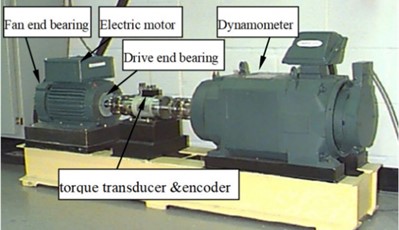
Fig. 2Fault waveform diagram
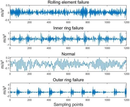
Table 1Description of CWRU bearing fault samples
Fault size / mm | State |
0.1778 | Rolling element failure |
0.1778 | Inner ring failure |
0.1778 | Normal |
0.1778 | Outer ring failure |
0.3556 | Rolling element failure |
0.3556 | Inner ring failure |
0.3556 | Outer ring failure |
0.5334 | Rolling element failure |
0.5334 | Inner ring failure |
0.5334 | Outer ring failure |
Divide ten different types of bearing fault signals into 50 sets of test set samples and 50 sets of training set samples. Due to the complexity of the vibration signal, the sample is preprocessed using VMD method, and several intrinsic mode components are obtained after decomposition. Taking the rolling element fault signal as an example, different pre-decomposition modes are selected for VMD, in which the penalty factor a takes the default value 2000. The main difference of different modes lies in the difference of the central frequency. According to the VMD algorithm, the central frequency of each IMF component obtained from the VMD of the vibration signal will be distributed from low frequency to high frequency. If you want to obtain the optimal preset scale , the center frequency of the last order IMF component should be the maximum for the first time. Table 2 shows the central frequencies of each IMF component under different modes.
As can be seen from Table 2, the minimum value of the central frequency is taken from the initial preset scale , and the maximum value of the central frequency tends to be stable when and . In order to prevent the mode numberof VMD from being too large and over-decomposing, thevalue selected in this paper is 4.
Table 2Center frequency after VMD when taking different k values
Preset scale | Center frequency | |||||||
IMF1 | IMF2 | IMF3 | IMF4 | IMF5 | IMF6 | IMF7 | IMF8 | |
= 2 | 25 | 545 | ||||||
= 3 | 25 | 250 | 720 | |||||
4 | 25 | 250 | 545 | 940 | ||||
5 | 25 | 250 | 545 | 720 | 940 | |||
6 | 25 | 250 | 350 | 545 | 720 | 940 | ||
7 | 25 | 250 | 350 | 545 | 720 | 940 | 1165 | |
8 | 25 | 250 | 350 | 545 | 570 | 720 | 940 | 1165 |
Taking the rolling element fault signal with a fault size of 0.1778mm as an example, the decomposed time-domain and frequency spectrum are shown in Fig. 3. From the time-domain graph, it can be seen that the VMD algorithm can decompose the original signal into multiple intrinsic mode components with different amplitudes through its built-in filtering algorithm. Observing the spectrum graph, it can be seen that the spectra of each component have obvious peaks, and there is no situation where multiple peaks appear simultaneously, avoiding mode mixing and boundary effects. From this, it can be seen that the VMD algorithm can effectively preprocess signals and improve the accuracy of subsequent work.
Fig. 3Time domain and frequency spectrum after VMD
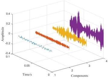
a) Time domain diagram after VMD
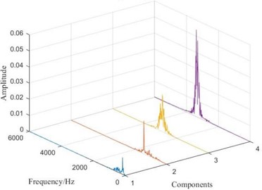
b) Spectrum after VMD
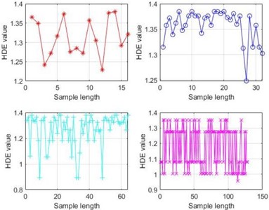
Use the HDE method to extract features from the decomposed multiple intrinsic mode components. The parameters in HDE affect the size of the extracted entropy and the overall effect. In order to determine the sensitivity of HDE to the original signal under different parameters, the average and standard deviation at different levels are calculated, and the coefficient of variation is introduced to determine the degree of node dispersion. The coefficient of variation is equal to the standard deviation/mean. As defined, the smaller the coefficient of variation, the higher the stability of the signal [18]. Fig. 4 shows the size of HDE entropy values under different parameters, while Tables 3 to 6 provide the coefficient of variation of HDE entropy values under different parameters.
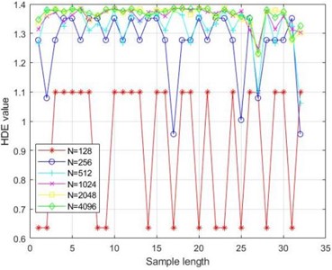
Due to the characteristics of the HDE algorithm, the final extracted sample length is . If the length parameter is set too small, the extracted entropy value is too small to be meaningful for discussion. If it is set too large, it will lead to excessive extraction, resulting in an invalid entropy value. Therefore, when discussing the sample length parameter , setting the range to [4, 7] will result in extracted entropy sample lengths of 16, 32, 64, and 128. From Fig. 4(a), it can be seen that when the sample length is 16 and 32, the entropy values are distributed within the [1.2, 1.4] range, while larger sample lengths only cause the entropy value to fluctuate and increase. From Table 3, it can be seen that the coefficient of variation is the smallest when the sample length parameter is 5, which also represents that the signal is most stable when the extracted sample length is 32. From Fig. 4(b), it can be seen that different lengths of original samples also affect the size and stability of the final extracted entropy. When the length of the original sample is , HDE tends to stabilize. Combined with Table 4, it can be seen that when the length of the original sample is 1024, the coefficient of variation is the smallest and the entropy value is also the most stable.
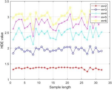
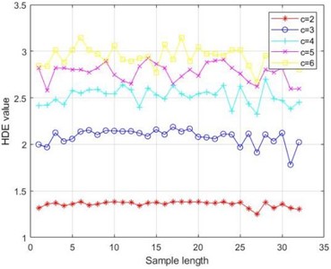
The different embedding dimensions and category also affect the performance of HDE. From Fig. 4(c), it can be seen that as increases, the fluctuation of entropy value increases. From Table 5, it can also be seen that when , the coefficient of variation is the smallest and the entropy value is the most stable. Therefore, the optimal embedding dimension is chosen; Similarly, by observing Fig. 4(d) and Table 6, the optimal number of categories can be obtained.
Fig. 4Entropy values under different conditions
a) Different entropy extraction sample lengths
b) Different original sample lengths
c) Different embedding dimensions
d) Different categories
In order to improve the accuracy of extraction, first extract the entropy information sample from the signal that has not been decomposed by VMD, and then use this sample as a benchmark to perform secondary extraction on the decomposed intrinsic mode components. The HDE parameters selected in this article are: original sample length , embedding dimension , number of categories , and sample length parameter . Due to secondary extraction, the length of each extracted sample increased from 32 to 64. The feature sample set extracted under this parameter is 100×64. In order to compare the effectiveness of the HDE method, the hierarchical range entropy (HRE) and hierarchical sample entropy (HSE) under the same parameters were also used for feature sample extraction. HDE is similar to HRE and HSE, which integrates range entropy and sample entropy on the basis of hierarchical entropy. The difference lies in the different calculation methods for signal sequences, resulting in different sets of extracted feature data. Taking the rolling element fault signal with a fault size of 0.1778 mm as an example, Fig. 5 shows a comparison of three entropy values.
Table 3Coefficient of variation for different entropy extracted sample lengths n
Sample length parameter | Coefficient of variation |
4 | 0.0043 |
5 | 0.0023 |
6 | 0.0396 |
7 | 0.0376 |
Table 4Coefficient of variation for different original sample lengths N
Original sample lengths parameter | Coefficient of variation |
128 | 0.1154 |
256 | 0.0286 |
512 | 0.0134 |
1024 | 0.0023 |
2048 | 0.0029 |
4096 | 0.0027 |
Table 5Coefficient of variation for different embedding dimensions m
Embedding dimensions parameter | Coefficient of variation |
2 | 0.0023 |
3 | 0.0053 |
4 | 0.0135 |
5 | 0.0146 |
6 | 0.0113 |
Table 6Coefficient of variation for different categories c
Categories parameter | Coefficient of variation |
2 | 0.0023 |
3 | 0.0079 |
4 | 0.0054 |
5 | 0.0044 |
6 | 0.0071 |
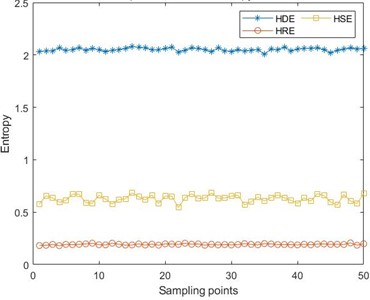
The entropy value can reflect the complexity of the bearing vibration signal, and the larger the entropy value, the higher the complexity of the vibration signal it represents. From the figure, it can be seen that after taking the mean of the extracted 100×64 feature samples, although the samples extracted by the HRE method have stability, their entropy values are between [0, 0.5], which cannot reflect the characteristics of the original fault signal well; The entropy value extracted by HSE method has increased compared to HRE, but its entropy value exhibits significant volatility, which is not conducive to the final fault classification; The entropy value extracted by the HDE method has high stationarity, and the entropy value is also larger than the other two extraction methods, indicating that this method can better demonstrate the complexity of signal features, which is beneficial for subsequent signal processing. To further demonstrate the effectiveness of the HDE method, Pearson correlation coefficient analysis was performed on the feature samples extracted by the three entropy extraction methods under four fault states with a fault size of 0.1778 mm. The results are shown in Fig. 6.
Fig. 5Comparison chart of three entropy values
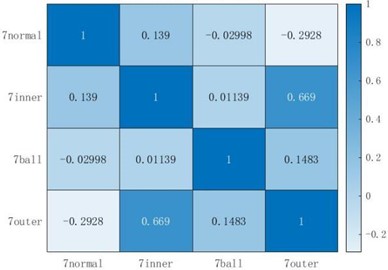
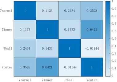
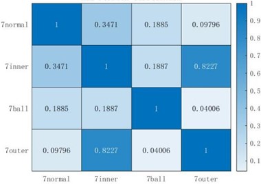
The Pearson correlation coefficient measures the correlation between the two, with a value range of [–1, 1]. After taking the absolute value of the correlation coefficient, the larger the value, the more relevant the two are. Comparing Fig. 6(a) and Fig. 6(b), it can be seen that the features extracted by HDE and HRE have a high correlation with both inner-outer faults, reaching above 0.6. However, for other types of faults, such as normal-ball faults, inner-ball faults, HDE Pearson correlation coefficients are much smaller than those of the HRE method, with only 0.02998 and 0.01139, while the HRE method only shows a small correlation when comparing ball-outer faults, and the correlation between other faults is not much different from that of the HDE method; Comparing three figures, it can be seen that the correlation between HSE and the extracted samples of inner-outer faults reaches 0.8227, which is much higher than the other two types of entropy values, indicating that the entropy values extracted by HSE for these two types of faults are highly correlated, which is not conducive to the final fault classification. The samples extracted by HSE showed good non correlation between normal-outer faults, as well as between outer-ball faults, but the non correlation between other faults was far inferior to the other two entropy values. In summary, the entropy extracted by HDE has better non correlation between each fault type compared to the other two methods, which can make the final fault diagnosis more accurate.
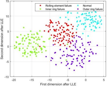
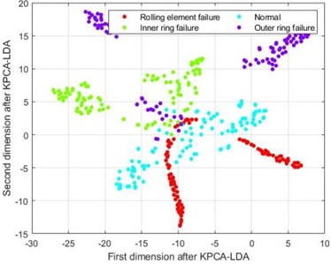
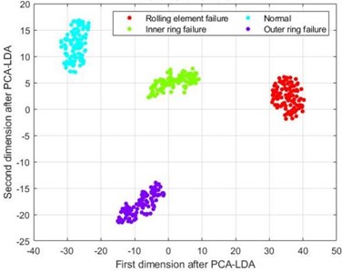
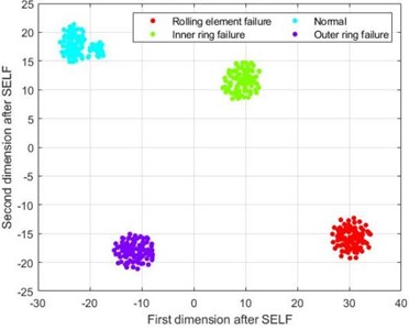
After feature extraction of the fault signal, the semi-supervised local fisher discriminant analysis (SELF) method was used to reduce its dimensionality. The weight coefficient of the SELF method, the reduced vector length , and the vector length obtained after SELF processing were reduced from 100×64 to 100×32. For comparative analysis, the entropy data extracted by HRE was also subjected to dimensionality reduction using LLE, KPCA combined with LDA, and PCA combined with LDA. Taking the feature samples under four fault states with a fault size of 0.1778 mm as an example, the t-SNE scatter plots of the reduced samples are shown in Fig. 7.
Although the four types of fault samples in Fig. 7(a) have a certain distribution pattern after dimension reduction using the LLE method, their various fault sample points are relatively scattered, and there is no clear boundary between different types of faults. The samples in Fig. 7(b), after dimensionality reduction using the KPCA-LDA method, although the sample points of various types of faults have a certain degree of aggregation compared to the LLE method, there is a mixture of different lengths in the four types of fault samples, and there is a significant separation phenomenon between the outer ring fault and rolling element fault samples, which greatly affects the accuracy of the final fault classification. From Fig. 7(c), it can be seen that the data after dimensionality reduction using PCA-LDA method has a clear boundary for four different types of faults, and there is no mixing of feature samples for each type; The four fault categories in Fig. 7(d) are similar to those in Fig. 7(c), with clear boundaries. However, the clustering degree of the data samples in Fig. 7(d) is closer than that in Fig. 7(c), indicating that the data samples after SELF dimensionality reduction can effectively distinguish different types of fault sample types, and the numerical values of different types of samples are divided into a certain range, resulting in higher discrimination between different types of samples and better fault diagnosis classification.
Fig. 6Pearson correlation coefficient chart
a) HDE Pearson correlation coefficient
b) HRE Pearson correlation coefficient
c) HSE Pearson correlation coefficient
Input the training and testing sets with a length of 100×32 obtained after dimensionality reduction into the least squares support vector machine optimized by particle swarm optimization for training and recognition. The optimization range of the regularization parameters and kernel parameters in the least squares support vector machine is set to [1, 200], the number of iterations is 10, and the maximum and minimum velocities of the particle swarm are 10 and –10. The least squares support vector machine performs 50 internal cross validations during fault classification of samples. The optimal parameter combination and accuracy obtained after training and testing the classification model are shown in Table 7. In order to demonstrate the effectiveness of this method, three entropy extraction methods and three data dimensionality reduction methods were combined to form a total of 12 methods for fault diagnosis. Table 7 also shows the classification accuracy of feature sample sets extracted by other methods in the model.
From the classification accuracy of LSSVM, we can see that for the three different entropy extraction methods, the correlation between the feature samples of different fault types is smaller under the HDE entropy extraction method, so it is easier to distinguish different fault types. From the final accuracy, we can see that after different dimensionality reduction methods, HDE method has higher accuracy than the other two entropy extraction methods; for different dimensionality reduction methods, the accuracy of SELF method is higher than that of the other three methods, which also proves the superiority of the semi-supervised local Fisher discrimination method proposed in this paper.
In order to further demonstrate the effectiveness of the method proposed in this paper, the deep learning classifier of deep extreme learning machine (DELM) is selected to compare again. This method effectively combines autoencoder with extreme learning machine to form a deep neural network structure. It combines the advantages of autoencoder and extreme learning machine, and makes use of the feature learning ability of autoencoder and the fast training characteristics of extreme learning machine, it can better extract the advanced features of data in depth structure, so as to improve the modeling ability of complex data, and can overcome some shortcomings of traditional deep neural network training, such as long-time training, gradient disappearance and so on. Thus, the training efficiency and the generalization ability of the model are improved.
Fig. 7t-SNE visualization diagram
a) t-SNE graph after LLE
b) t-SNE graph after KPCA-LDA
c) t-SNE graph after PCA-LDA
d) t-SNE graph after SELF
Table 7CWRU data classification accuracy of LSSVM
Entropy extraction method | Dimension reduction method | Regularization parameter | Kernel parameter | Classification accuracy (%) |
HDE | SELF | 80.33 | 9.84 | 100 |
PCA-LDA | 84.43 | 1.14 | 96.8 | |
KPCA-LDA | 9.64 | 0.43 | 90.8 | |
LLE | 6.31 | 2.36 | 81.4 | |
HRE | SELF | 10.66 | 4.31 | 100 |
PCA-LDA | 28.55 | 0.14 | 95 | |
KPCA-LDA | 46.78 | 0.10 | 86.8 | |
LLE | 5.64 | 9.21 | 65 | |
HSE | SELF | 3.26 | 6.44 | 99.6 |
PCA-LDA | 47.67 | 0.10 | 93.2 | |
KPCA-LDA | 81.73 | 1.45 | 84.8 | |
LLE | 69.98 | 9.68 | 79.2 |
Similarly, the reduced samples are input into the depth extreme learning machine optimized by the optimization algorithm for training and recognition. The optimization range of weight parameters of depth extreme learning machine is set to [–10, 10], the number of iterations is 50, and the number of iterative populations is 20. The deep extreme learning machine performs 50 internal cross-validation in the process of sample fault classification. The diagnostic accuracy of 12 fault diagnosis methods in the optimized DELM model is shown in Table 8. As can be seen from Table 8, the accuracy of three different entropy extraction methods after dimensionality reduction by SELF method has reached 100 %, indicating the advantage of SELF method in data dimensionality reduction. For the same dimensionality reduction method, the accuracy of HDE entropy extraction method is also higher than that of other entropy extraction methods, which shows the accuracy of the proposed method. Overall, the optimized DELM method has higher classification accuracy than LSSVM method, and can better classify samples.
Table 8CWRU data classification accuracy of DELM
Entropy extraction method | Dimension reduction method | Weight parameter | Classification accuracy (%) |
HDE | SELF | 0.4520 | 100 |
PCA-LDA | 0.2680 | 97.4 | |
KPCA-LDA | 1.3260 | 92.6 | |
LLE | 0.5640 | 85.8 | |
HRE | SELF | 0.4660 | 100 |
PCA-LDA | 0.4340 | 96.8 | |
KPCA-LDA | 1.3320 | 88.2 | |
LLE | 0.8860 | 68.4 | |
HSE | SELF | 0.4420 | 100 |
PCA-LDA | 0.4380 | 94.2 | |
KPCA-LDA | 1.2460 | 86.4 | |
LLE | 0.4180 | 82.6 |
4.2. Southeast University (SEU) dataset
Due to the fact that the Case Western Reserve University bearing dataset achieved high accuracy in extracting feature vectors using three entropy extraction methods and then reducing the dimensionality through SELF, both HRE-SELF and HDE-SELF achieved 100 % accuracy. Therefore, in order to better demonstrate the accuracy of the method proposed in this article, further experiments will be conducted on the dataset of Southeast University. The Southeast University (SEU) dataset is a gearbox dataset provided by Southeast University [19], and the fault test bench is shown in Fig. 8. This dataset consists of two sub datasets, including the bearing dataset and the gear dataset. The bearing dataset simulates five bearing operating states under two different operating conditions, namely 20 Hz (1200 r/min) - unloaded 0 V (0 N/m) and 30 Hz (1800 r/min) - loaded 2 V (7.32 N/m). The specific fault types are shown in Table 9, and the fault wave-forms are shown in Fig. 9.
Fig. 8Southeast University bearing test bench

Table 9Description of SEU bearing fault samples
Speed load situation | Fault Type | Fault description |
20 Hz-0 V | Ball | Cracks appear on the ball bearings |
Combination | Cracks appear on the inner and outer rings | |
Normal | Healthy operation status | |
Inner | Cracks appear in the inner ring | |
Outer | Cracks appear on the outer ring | |
30 Hz-2 V | Ball | Cracks appear on the ball bearings |
Combination | Cracks appear on the inner and outer rings | |
Normal | Healthy operation status | |
Inner | Cracks appear in the inner ring | |
Outer | Cracks appear on the outer ring |
Fig. 9Fault waveform diagram
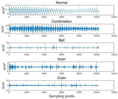
a) 20 Hz-0 V fault signal
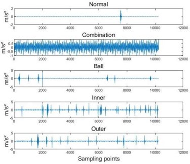
b) 30 Hz-2 V fault signal
Similar to the previous text, ten different types of fault signals are divided into training and testing sets, preprocessed through VMD decomposition, and their HDE entropy values are extracted. The HDE parameter settings are the same as the previous text, but will not be further elaborated here. Further perform dimensionality reduction on the extracted 100×64 entropy samples. Taking 5 types of fault samples with a speed load condition of 20 Hz-0 V as an example, Fig. 10 show the t-SNE scatter plots of four dimensionality reduction methods under HDE method.
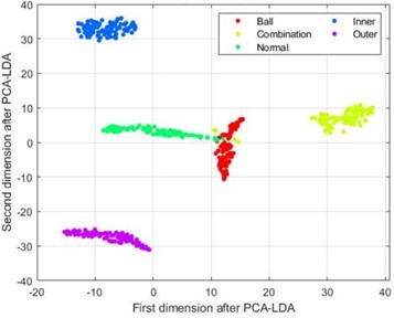
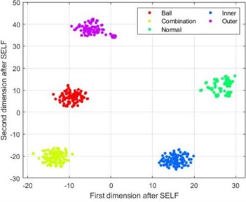
From Fig. 10(a) and 10(b), it can be seen that the feature samples after dimensionality reduction using LLE and KPCA-LDA methods still exhibit hybridization, and various types of fault samples are relatively scattered without good discrimination; The PCA-LDA method in Fig. 10(c) performs much better in reducing the dimensionality of the samples compared to the previous two methods, but there is still a situation of mixed sample points in the dimensionality reduction of the first three types of fault samples; From Fig. 10(d), it can be seen that the sample points of each fault type in the data after dimensionality reduction using the SELF method are mapped to separate regions, with good discrimination.
Input the dimensionality reduced data samples into the least squares support vector machine optimized by particle swarm optimization for training and testing. Table 10 shows the optimal parameter combinations and classification accuracy of 12 methods. From the previous analysis and the data in the table, it can be seen that the HDE entropy extraction method has a smaller correlation between the extracted samples compared to the other two entropy extraction methods, which makes its accuracy higher than the other two entropy values after the same method of dimensionality reduction, verifying the previous analysis; From the previous analysis, it can be seen that among the four dimensionality reduction methods, the discrimination between datasets under SELF dimensionality reduction is higher, which is also reflected by the final classification accuracy. The accuracy of the HDE combined with SELF dimensionality reduction method reached 98.2 %, verifying the effectiveness of the HDE-SELF method proposed in this paper.
Fig. 10t-SNE visualization diagram
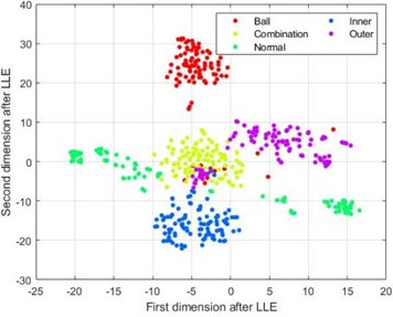
a) t-SNE graph after LLE
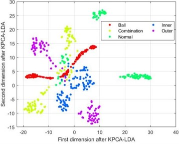
b) t-SNE graph after KPCA-LDA
c) t-SNE graph after PCA-LDA
d) t-SNE graph after SELF
Table 10SEU data classification accuracy
Entropy extraction method | Dimension reduction method | Regularization parameter | Kernel parameter | Classification accuracy |
HDE | SELF | 58.04 | 18.56 | 98.2 |
PCA-LDA | 75.50 | 1.67 | 96.4 | |
KPCA-LDA | 73.78 | 1.33 | 89.2 | |
LLE | 25.47 | 9.15 | 93.2 | |
HRE | SELF | 96.86 | 11.36 | 93.8 |
PCA-LDA | 77.51 | 0.1 | 91.8 | |
KPCA-LDA | 76.48 | 0.1 | 87.6 | |
LLE | 23.62 | 8.41 | 86 | |
HSE | SELF | 58.59 | 76.20 | 95.8 |
PCA-LDA | 30.54 | 0.1 | 93.2 | |
KPCA-LDA | 83.57 | 1.01 | 86.6 | |
LLE | 97.27 | 6.71 | 93 |
As mentioned above, the DELM method is used to classify SEU fault samples. As can be seen from Table 11, the final fault diagnosis accuracy of the samples processed by HDE and SELF is the highest, reaching 99.6 %. The other two entropy extraction methods also achieve high accuracy in the case of SELF processing, which once again proves the effectiveness of the SELF method. For different entropy extraction methods, the accuracy of HDE method is also higher than that of the other two methods. Generally speaking, the data processed by the HDE-SELF method proposed in this paper has high classification accuracy, which also shows the effectiveness of the method.
Table 11SEU data classification accuracy of DELM
Entropy extraction method | Dimension reduction method | Weight parameter | Classification accuracy (%) |
HDE | SELF | 0.4740 | 99.6 |
PCA-LDA | 0.1620 | 97.2 | |
KPCA-LDA | 1.1660 | 90.2 | |
LLE | 0.2880 | 94.6 | |
HRE | SELF | 0.4420 | 98 |
PCA-LDA | 0.6080 | 92.4 | |
KPCA-LDA | 1.0300 | 88 | |
LLE | 0.3560 | 87.8 | |
HSE | SELF | 0.4580 | 98.4 |
PCA-LDA | 0.4780 | 94.2 | |
KPCA-LDA | 1.0440 | 88.6 | |
LLE | 0.1920 | 93.8 |
5. Conclusions
This article proposes a bearing fault diagnosis method that combines Hierarchical Discrete Entropy (HDE) with Semi Supervised Local Fisher Discriminant Analysis (SELF) dimensionality reduction. The conclusions are as follows:
1) Compared to the other two entropy extraction methods, the HDE method extracts feature samples with lower correlation, which enables the HDE method to achieve higher accuracy in classifying feature samples.
However, the parameter selection problem in entropy extraction methods has always been a problem that needs to be solved. This article only uses the method of comparing the entropy values obtained after setting different parameters to determine the optimal parameters. However, different parameter combinations can also affect the size and stationarity of entropy extraction samples. Therefore, whether an optimization algorithm can be found to optimize its parameters and find the optimal parameter combination is a new research point.
2) The SELF dimensionality reduction method uses a semi supervised approach to reduce the dimensionality of labeled samples. Compared to supervised dimensionality reduction methods such as LDA and unsupervised dimensionality reduction method LLE, the discrimination between data samples after SELF dimensionality reduction is higher, resulting in higher accuracy.
For the Case Western Reserve University dataset and Southeast University dataset, the final accuracy of the HDE-SELF method proposed in this paper is the highest, which proves the effectiveness of this method. In future research, we will also incorporate deep learning methods into the dimensionality reduction process to achieve better results.
References
-
H. Huang and J. Weiand Z. Ren, “Rolling bearing fault diagnosis based on imbalanced sample characteristics oversampling algorithm and SVM,” Journal of Vibration and Shock, Vol. 39, No. 10, pp. 65–74, May 2020, https://doi.org/10.13465/j.cnki.jvs.2020.10.009
-
W. Wang, F. Yuan, and Z. Liu, “Sparsity discriminant preserving projection for machinery fault diagnosis,” Measurement, Vol. 173, p. 108488, Mar. 2021, https://doi.org/10.1016/j.measurement.2020.108488
-
J. Li, X. Yao, X. Wang, Q. Yu, and Y. Zhang, “Multiscale local features learning based on BP neural network for rolling bearing intelligent fault diagnosis,” Measurement, Vol. 153, No. 1, p. 107419, Mar. 2020, https://doi.org/10.1016/j.measurement.2019.107419
-
Y. Xue, C. Wen, Z. Wang, W. Liu, and G. Chen, “A novel framework for motor bearing fault diagnosis based on multi-transformation domain and multi-source data,” Knowledge-Based Systems, Vol. 283, p. 111205, Jan. 2024, https://doi.org/10.1016/j.knosys.2023.111205
-
W. Wei and X. Liu, “Fault diagnosis of S700K switch machine based on EEMD multiscale sample entropy,” Journal of Central South University (Science and Technology), Vol. 50, No. 11, pp. 2763–2772, Nov. 2019.
-
W. Yang, P. Zhang, and H. Wang, “Gear fault diagnosis based on multiscale fuzzy entropy of EEMD,” Journal of Vibration and Shock, Vol. 34, No. 14, pp. 163–167, Jul. 2015, https://doi.org/10.13465/j.cnki.jvs.2015.14.028
-
Y. Jiang, C.-K. Peng, and Y. Xu, “Hierarchical entropy analysis for biological signals,” Journal of Computational and Applied Mathematics, Vol. 236, No. 5, pp. 728–742, Oct. 2011, https://doi.org/10.1016/j.cam.2011.06.007
-
F. Zhou, X. Yang, and J. Shen, “Modifier multivariate hierarchical fluctuation dispersion entropy and its application to the fault diagnosis of rolling bearings,” Journal of Vibration and Shock, Vol. 40, No. 22, pp. 167–174, Nov. 2021, https://doi.org/10.13465/j.cnki.jvs.2021.22.023
-
Y. Li, H. Song, and P. Li, “Application of improved dispersion entropy to fault detection of Axle-Box bearing in train,” Journal of Vibration, Measurement and Diagnosis, Vol. 43, No. 2, pp. 304–311, Apr. 2023, https://doi.org/10.16450/j.cnki.issn.1004-6801.2023.02.014
-
Q. Li, “New sparse regularization approach for extracting transient impulses from fault vibration signal of rotating machinery,” Mechanical Systems and Signal Processing, Vol. 209, p. 111101, Mar. 2024, https://doi.org/10.1016/j.ymssp.2023.111101
-
J. Zheng, T. Liu, and R. Meng, “Generalized composite multiscale permutation entropy and PCA based fault diagnosis of rolling bearings,” Journal of Vibration and Shock, Vol. 37, No. 20, pp. 61–66, Oct. 2018, https://doi.org/10.13465/j.cnki.jvs.2018.20.010
-
Y. Zhou, S. Yan, Y. Ren, and S. Liu, “Rolling bearing fault diagnosis using transient-extracting transform and linear discriminant analysis,” Measurement, Vol. 178, No. 3, p. 109298, Jun. 2021, https://doi.org/10.1016/j.measurement.2021.109298
-
J. Wu, Q. Zhou, and L. Duan, “Recommendation attack detection using semi-supervised fisher discriminant analysis,” Journal of Chinese Computer Systems, Vol. 41, No. 12, pp. 2649–2656, Dec. 2020.
-
L. Jiang, J. Xuan, and T. Shi, “Feature extraction based on semi-supervised kernel Marginal Fisher analysis and its application in bearing fault diagnosis,” Mechanical Systems and Signal Processing, Vol. 41, No. 1-2, pp. 113–126, Dec. 2013, https://doi.org/10.1016/j.ymssp.2013.05.017
-
M. Sugiyama, T. Idé, S. Nakajima, and J. Sese, “Semi-supervised local Fisher discriminant analysis for dimensionality reduction,” Machine Learning, Vol. 78, No. 1-2, pp. 35–61, Jul. 2009, https://doi.org/10.1007/s10994-009-5125-7
-
F. Nie, Z. Wang, R. Wang, Z. Wang, and X. Li, “Adaptive local linear discriminant analysis,” ACM Transactions on Knowledge Discovery from Data, Vol. 14, No. 1, pp. 1–19, Feb. 2020, https://doi.org/10.1145/3369870
-
T. Zhang, Y. Chen, and Y. Chen, “Hierarchical dispersion entropy and its application in fault diagnosis of rolling bearing,” Journal of Vibroengineering, Vol. 24, No. 5, pp. 862–870, Aug. 2022, https://doi.org/10.21595/jve.2022.22354
-
Case Western Reserve University (CWRU) Bearing Data Center, https://csegroups.case.edu/bearingdatacenter/pages/download-data-file/.
-
S. Shao, S. Mcaleer, R. Yan, and P. Baldi, “Highly accurate machine fault diagnosis using deep transfer learning,” IEEE Transactions on Industrial Informatics, Vol. 15, No. 4, pp. 2446–2455, Apr. 2019, https://doi.org/10.1109/tii.2018.2864759
About this article

The authors have not disclosed any funding.
The datasets generated during and/or analyzed during the current study are available from the corresponding author on reasonable request.
Yongqi Chen: conceptualization. Qian Shen: data curation. Qian Shen: formal analysis. Liping Huang: methodology. Tang Zhang: writing-original draft preparation. Zhongxing Sun: writing-review and editing.
The authors declare that they have no conflict of interest.
