Abstract
Utilization of airborne Inverse-Synthetic-Aperture-Radar (ISAR) for detection of moving targets on the sea surface is studied in this paper. In order to systematically analyze the characterization of radar imaging in the presence of both motion and observation uncertainty of a target, this study incorporates the Bayes-PRM multi-query algorithm for fusing ISAR multi-sensing information. The algorithm isochronously samples the physical quantities, such as UAV position, altitude, pitch angle, and velocity as a sequence of multivariate groups, and converts the time-series data of the trajectories into distributional features in graph theory. The coupled edge weights and Alternating Direction Method of Multipliers (ADMM) are introduced through the coupling framework combined with the ambient graph. With ADMM, the quadratic penalty term is used to achieve a simple linear function, and subproblems involving amplitude, linear velocity, and yaw angle can be embedded in a sequential solution scheme. The quality of the primal and dual solutions is then improved in an iterative manner to achieve vector analysis of the UAV. The potential maneuvering region of the target is fitted to a Gaussian-Wiener stochastic movement model, which in turn yields the detection expectation through point set coverage. By analyzing the tracking simulation results and diffraction theory, the experimental results are transformed into a function of the UAV multi-vector, and the angular linearization model of the multi-vector under the radar image is developed, which solves the optimal elevation angle and the optimal path for the maximum scanning radius of the airborne radar. The nominal trajectory of the UAV is effectively obtained, which confirms the improvement of the credibility of ISAR in target detecting. Through the proposed model, the results of object detection accuracy were improved.
1. Introduction
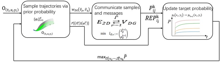
Featuring advantages such as high mobility and high positioning accuracy, UAV search has been widely used in various fields including military, surveillance, environmental monitoring and disaster management [1]. Among the many applications of UAVs, using them for high-precision and comprehensive surveillance of vast sea areas has attracted much attention in recent years [2]. Inverse synthetic aperture radar (ISAR) on UAVs takes full advantage of the maneuverability and advanced radar capabilities of UAVs for detecting, tracking, and monitoring maritime targets, providing a significant improvement over traditional methods in terms of coverage, flexibility, and efficiency [3]. However, the dynamic nature of the maritime environment, coupled with the motion of UAVs and targets, poses significant challenges for radar imaging and target characterization [4]. ISAR is particularly effective when the target is in motion, so one of the main challenges in UAV ISAR imaging is the uncertainty of target motion and UAV observation capabilities [5]. To systematically analyze radar imaging under these conditions [6], researches have integrated the PRM probabilistic roadmap algorithm for path planning [7]. As being more mature than RRT, PSO and other algorithms, PRM has been more widely used in the field of path planning in recent years [8]. In order to further improve the analysis, the proposed CTop-PRM is implemented on the basis of the PRM algorithm which can effectively improve the efficiency and complexity of the algorithm, and provides a robust framework for target detection and characterization of new sparse roadmaps [9]. It is necessary to comprehensively consider the characteristics of UAV motion and imaging devices [10], introduce coupled edge weights in conjunction with the environment graph [11], and utilize graph theory to convert the time series data of UAV trajectories into distributional characteristics [12] Stochastic time series can be represented through neural networks and autoregressive moving average models, meaning that the series can be explained by its own past or lagged values as well as random disturbance terms [13]. If the series is stationary, its behavior does not change over time, then we can predict its future based on its past behavior [14]. Variables such as UAV position, velocity, and pitch angle are involved, and these sub-problems are embedded into a sequential solution scheme through the ADMM algorithm [13]. The quality of the original and pairwise solutions is iteratively improved [15], thus increasing the accuracy of the UAV vector analysis [16]. Previous studies used the mapping of coupled workspace nodes with copies of the environment graph to ensure that the orientation of the moving subject at the path nodes is unrestricted [17], but the mapping cost was not considered [18]. Bayesian estimation of spatial multi-location and Bayesian detection with feedback have also been proposed in the presence of system uncertainty and external disturbances [19]. The optimal stopping time is optimized based on the local energy detection results so that the target can be found again and continue to track the target in case of loss [20]. However, the flow structure where energy is dissipated is not considered [21], which can lead to perception delay and false alarms [22]. Based on the above analysis, this paper proposes the Bayes-PRM multi-query algorithm that fuses ISAR multi-sensing information. The potential maneuver region of the target is modeled with a Gauss-Wiener stochastic motion model to provide a probabilistic framework for estimating the target detection region. The model is combined with a point set coverage technique to derive the expected detection area. The analysis of tracking simulation results and graph-theoretic diffraction is transformed into a function of UAV multi-vectors, resulting in more accurate vector analysis and target tracking detection. This approach not only enhances the detection capability of UAV-based ISAR systems, but also provides a powerful framework for real-time maritime surveillance.
2. Proposed model
2.1. Initial static prior probabilities
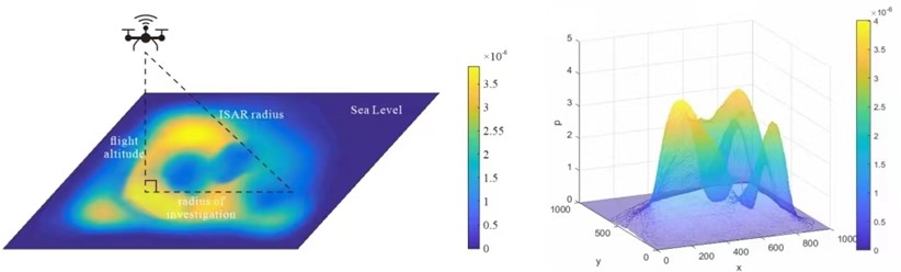
The prior probability of a target appearing at different locations in the search region under maneuvering conditions is first generated by normalizing the heat map based on a given characterization of the historical pattern. denotes the coordinate position of , , . Record the detection space consisting of all points as , , denotes the thermal value matrix, denotes the thermal value of . Use the heat value to build a normalized prior probability model. represents the probability of a target appearing at position . The computational model is shown in Eq. (1):
We calculate the prior probabilities for the motorized condition based on Eq. (1). The sum of all probabilities in the result is 1, and the distribution and variation are consistent with the heat map. The corresponding visualization of the normalized probability matrix is shown in Fig. 1.
Fig. 1Probability distribution of target occurrence after normalization
2.2. ISAR detection probability model
The UAV takes image every seconds, and at , has imaged for times:
The probability of UAV detecting a target in imaging is , and the path chosen through waypoint depends on information from previous and subsequent waypoints. denotes that the target lies within the detection range of the waypoints. Consider that the UAV must navigate through a sequence of spatial path points given by, where , . is the set of other UAV imaging information that the UAV is able to receive. The updated probability of achieving the target’s existence from the Bayesian criterion is calculated in Eq. (3) [6]:
According to the joint search target probability update model, the dynamic update formula of target existence probability at is described in Eq. (4):
2.3. Bayes-PRM based waypoint sequence planning
Bayes-PRM samples the ternary sequence of UAV detection routes , represent the time of the th waypoint, is the -coordinate and is the -coordinate. Based on the imaging intervals, the space is equidistant into a node graph, thus approximating a complete representation of the environment and obtaining a complete connectivity characterization of the configuration space. This method ensures that the sampling moments of the waypoints are identical for all the routes of the UAV facing the problem, and also ensures the temporal alignment properties of the problem for computing the dynamic time-varying a priori probabilities. The roadmap is built locally from a specific initial configuration, and then a feasible path can be obtained through graph search. The graph coupling framework forces the UAV to traverse the heading angles and derive the optimal heading angle based on the direction probability magnitude. Then introduce edge weights with a detection target in mind and minimize the penalty function . The set of points at these waypoints also constitute the decision variables of the optimization model.
Fig. 2Bayes-PRM algorithm deployed on UAVs
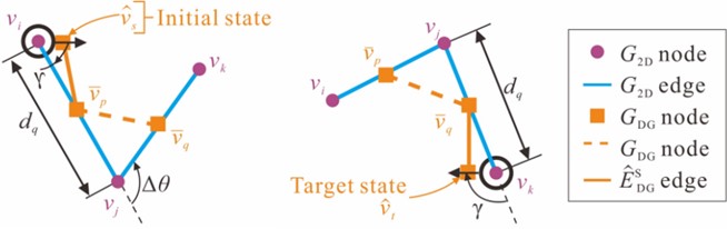
We use the algorithm to perform random sampling in the space to obtain a set of nodes or vertices . is a set of links or edges connecting pairs of nodes, i.e., feasible paths from the start node to the target node . , where the tail node is and the head node , each node can be described with spatial coordinates and , and the environment is represented by the graph [11].
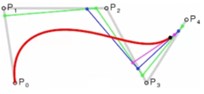
Coupling two copies of graph together, the turn cost is computed by transforming the graph into the dual graph by transforming the edges of the representative graph into nodes. is a bijective transformation that associates the representative edges in with the corresponding nodes in as shown in Fig. 3, . Assume that the UAV starts from , and arrives at the unique cost node . It is reoriented from the initial state along the corresponding edge in , with a change edge distance of , initially facing west at node at an angle to edge .
Upon reaching the final node, the cost of the new edge must include the traversal cost along the as well as the cost of reorientation to the final state . Its final desired state is located at node of and faces west at an angle to edge .
Fig. 3Graph coupling framework
Based on configuration space sampling, when each edge introduces a weight correlation factor, the edges are weighted by a cost function that takes into account traversal and turning costs. The coupled edge weight function is expressed as Eq. (5):
The traversal and reorientation cost of controlling the intelligent body traveling along distance is reoriented at by to align with edge . The traversal cost is given by . is the cost of rotation required to rotate . Consider that the UAV is located at at that moment, its probability value is , and the probability of moving to each position is respectively. According to the maneuvering law, the movement of the UAV should be consistent with the heat map. Therefore, the probability of moving to each position should be proportional to its corresponding probability value, satisfying Eq. (6):
The correction to the existence probability of the surrounding movement toward the location is expressed in Eq. (7):
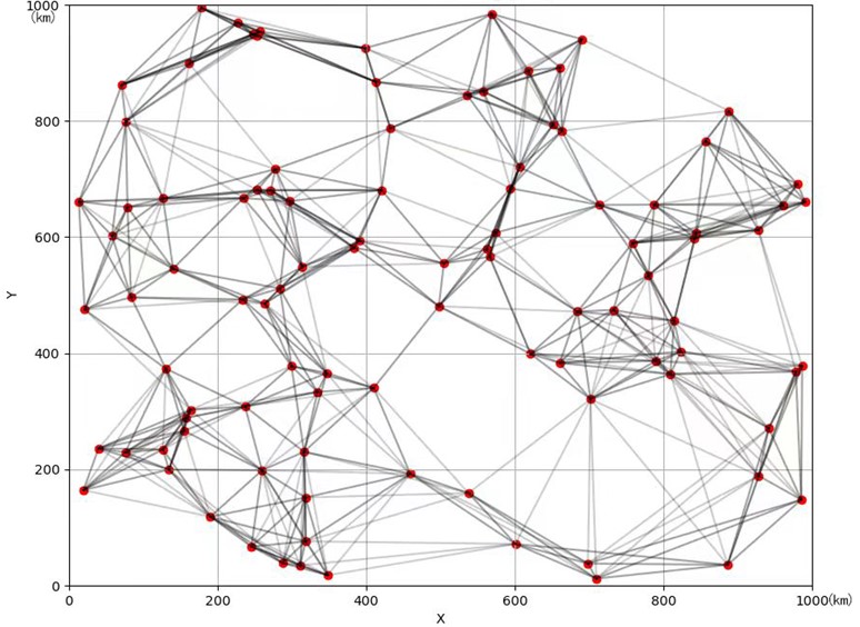
Connections are subsequently established between waypoints to form probabilistic routes, see Fig. 4.
Fig. 4Paths planned by Bayes-PRM
2.4. UAV vector analysis
The rotation matrix of the vector from the airframe coordinate system to the earth coordinate system is expressed in Eq. (8) [12]:
where, is the rotation matrix from (airframe coordinate system) to (earth coordinate system); is the roll angle rotating around the -axis, is the pitch angle rotating around the -axis, is the yaw angle rotating around the -axis, respectively. The above triangles are collectively called Euler’s angles (a set of three independent angular coefficients for determining the position of the fixed-point rotating rigid body). The dynamics of the UAV is modeled according to the Newton-Euler equations, and from Newton’s second law, we have:
Left-multiply the rotation matrix , and convert to the Earth coordinate system:
Set up unit vectors through the Earth’s coordinate system:
We combine the equations for the combined external force and velocity in the dynamic model:
By expressing the equation for attitude through Euler angles, the rate of change of attitude angle is related to the angular velocity of rotation of the airframe as follows:
Then:
In the case of small perturbations, the rate of the attitude angle change is approximately equal to the rotational angular velocity of the airframe, then:
2.5. ADMM-based solutions
Set ISAR phased array system with isotropic elements as , is a three-dimensional vector representing the position of the th sensor in the Cartesian coordinate system, and the unit vectors are , and , the association matrix is:
by connecting steering vectors , , .
The auxiliary variables , . Due to the nature of the ADMM, this property is built on real-valued and convex functions. In many ADMM applications, the augmented Lagrangian function is used for the definition of a single penalty parameter for all constraints. This algorithm utilizes two different penalty parameters and to minimize the sets of variables w and under constraints respectively. The solution to Eq. (12) is generated by imposing the kinematic model and vector constraints as individual subproblems of ADMM [16]:
By equationally constraining the coupling, applying the augmented Lagrangian of ADMM on Eqs. (20), (21) requires defining the penalty parameter:
In the scaled form of ADMM, [17]:
where is the weight of the squared error, and is responsible to control . By means of the residual convergence feature of the ADMM, it is observed that the constrained raw residuals converge to zero as .
3. Target maneuver model and multiple cruise detection
3.1. Target maneuver prediction model
Since the target carries out a wide range of maneuvers in the hotspot area, a suitable potential maneuver area needs to be constructed according to the maneuver characteristics. The acceleration is consistent within , and the Gaussian white noise sequence with the same variance . The target maneuvers to at time . is the velocity , and are the positions in the direction and direction respectively, at time :
3.2. Target transfer probability density function modeling
The potential maneuver region of the target within approximates a circular region centered on . The maximum error allowed for a velocity of is . The transfer probability density obeys a Gaussian distribution with and as the radius of the entire potential region, respectively, and is averaged over the points on the circle, as shown in Fig. 5.
Fig. 5Target transfer probability density function
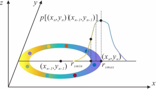
The target obeys a Gaussian distribution with the mean value of and the variance of after at position , as can be deduced from Eq. (27) (the same for ):
We assume that the estimated maneuvering speed is , and the angle between the speed direction and -axis is :
The transfer probability density function of the target position from to after is:
3.3. Waypoint detection expectations
The probability () that the coordinate in the region where the UAV detection range coincides with the target maneuvering range can be detected is [20]:
where is the existence probability that the target is located on coordinate at moment ; is the probability of target detection from ISAR images at moment . The probability that the target is located at a certain determined position among the detection range is . Then the detection probability is:
Based on the coverage situation on the detection area, we take as the coverage radius, and statistically generate the coverage of the waypoint . And the waypoint set covered by all waypoints is generated. Based on Bayes’ theorem, the th imaging distance can be represented as . And the UAV detection expectation is calculated followed:
4. System simulation results and analysis
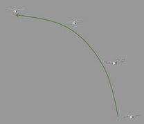
Fig. 6 shows the dynamic simultaneous navigation of waypoints in sequence considering coupling edge weights and turning costs.
In this paper, the UAV travel measurement is transformed into a study of the state of a controlled system, while vectorization can be modeled in Simulink to simulate and analyze the characteristic uncertainties of the system. The following three points are focused: 1) Dynamics Model: to establish the dynamics model of the UAV, including the equations of motion of the vehicle, attitude dynamics, etc. 2) State Estimation: to design the state estimator to obtain the system state information, such as the position, attitude, velocity, etc. 3) Simulation and Analysis: to conduct simulation experiments in Simulink to analyze the response, stability and performance of the system, and to optimize the control strategy.
Fig. 6Coupled weighting for dynamic synchronization of waypoints for navigation
a)
b)
c)
d)
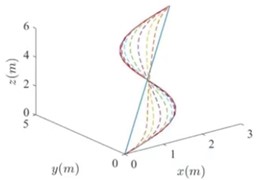
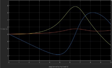
In order to verify the vector variation of UAV under state feedback control based on ADMM, the initial state of the UAV is set to [0, 0, 0], the initial pitch angular velocity is 10 rad/s, the initial position of the UAV is set to be in equilibrium, and the motion starts to increase its rotational angular velocity, the dynamic process of the vehicle is shown in Fig. 7(a). Combined with the flight dynamics vector equation, it can be concluded that the forces and moments generated by the wing are changed, and the vehicle, under the action of the unbalanced forces and moments, the linear velocities in the three directions are dispersed, in which the -direction velocities are changing rapidly, and the whole becomes an upward state as in Fig. 7(b). When the pitch angle speed is 20°, the vertical and longitudinal motion speeds of the vehicle change a large amount, and the lateral motion speed hardly changes; the pitch angle rate and the rise rate of the yaw angle rate are accelerated, as shown in Fig. 7(c) Therefore, it can be concluded that the pitch channel has strong coupling with the vertical and longitudinal velocities and weak coupling with the lateral velocity and yaw. From the perspective of measurement sensitivity and specificity, choosing the force and moment terms as control quantities, the maneuver coupling is smaller compared to directly using the rotational angular velocity as the maneuver quantity, thus proving the rationality of adopting the former as the base control quantity.
Fig. 7UAV nominal and state trajectories
a)
b)
c)
As shown in Figs. 8-9, the change of angular velocity directly affects the attitude angle of the UAV. The angular velocity is the time derivative of the attitude angle change, so when the angular velocity increases, the attitude angle changes faster. When the angular velocity decreases, the attitude angle changes slower. This change in attitude angle is usually caused by an adjustment in angular velocity. As the angular velocity changes, the UAV changes its attitude with some angular acceleration to reach the new angle value.
Accordingly, we introduce the ADMM algorithm, which imposes the kinematic model and vector constraints as a single subproblem of ADMM for a certain number of iterations. If there is still no significant convergence trend in the original residuals, is adjusted to accelerate to a feasible angular velocity solution . In contrast, if a feasible solution is obtained (with the original residuals equal to 0), can be reset to its initial value to explore other feasible solutions. With the help of this parameter updating strategy, the problems of slow convergence of local optima, early stopping and possible traps can be better mitigated. It is recommended to choose initial values of between 0.1 and 10 to produce good performance.
Fig. 8Variation of UAV attitude angle
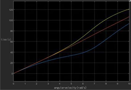
Fig. 9Variation of UAV angular velocity
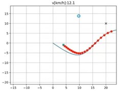
In order to test our algorithm on different configurations and scales, our algorithm is executed to solve for different scales of attitude angles , , . Comparing the method using standard LR and the ADMM-based algorithm to solve this situation, the computation time for each iteration is about 20 seconds. Observe the model position loop tracking by setting different penalty functions. The initial penalty parameter is set to 1 iteration process is shown in Fig. 10. When the penalty function is set too small, it will show harmonic-like fluctuation characteristics, and with the dynamic adjustment of and , so that the system residuals converge to 0, the position loop tracking tends to be stable and bounded. It was finally determined that stable high quality values were obtained in the iterations when is 0.25 and is 2.
The simulation certifies that the UAV has a small steady state error with good control accuracy, and the system response curve rise time is less than expected, the state variables converge quickly, and are tracked well once in a steady state. The waypoint dataset used in this study is provided from the laboratory, which is designed for the problem of detecting moving targets on the sea surface. The waypoint sequence detection algorithm for a real dynamic scene is set to have a UAV maneuvering radius of 10 km. The UAV on-board ISAR images the target area once every 20 seconds, covering a radius of 60 km.
In order to express the specific role of measurements, we set Sub-1: sea surface with multiple vessels sailing in close proximity; Sub-2: simultaneous presence of both large-range maneuvering and small-range maneuvering vessels; and Sub-3 marina with multiple types of vessels at berth. Compared to the detection results of 2D-Grating, CTRV (Constant Turn Rate and Velocity), Bayes-PRM algorithms in the sample library testing training algorithm as shown in Table 1, this study verifies the effectiveness of the proposed method through sampling imaging.
Fig. 10Model position loop tracking rendering
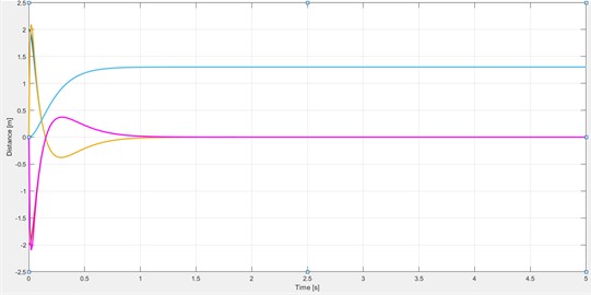
Table 1Waypoint sequence detection rate by 2D-Grating, CTRV, Bayes-PRM algorithms
Method | 2D-Grating | CTRV | Bayes-PRM |
Sub-1 | 81 % | 85.43 % | 99.28 % |
Sub-2 | 78.7 % | 54.6 % | 81.2 % |
Sub-3 | 77.52 % | 83.52 % | 86.48 % |
The accuracy of the improved Bayes-PRM algorithm is significantly higher than the other models, and further training on ISAR imaging detection under sea navigation conditions is conducted to verify the effectiveness of the algorithm.
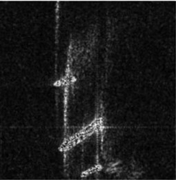
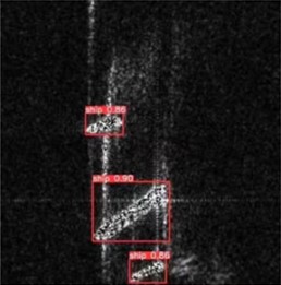
Fig. 11 shows the effectiveness of the improved algorithm verified by sampled imaging after experimental operation with ISAR on board. A dynamic scene of adjacent sailing of multiple ships was established from the dataset, with the detection probability of the independent sailing vessel at the top being 85 %, the detection probability of the large vessel in the middle being 90 %, and the detection probability of the partially obstructed vessel at the bottom being 86 %. The detection results proved the effectiveness of the algorithm.
Fig. 11a) Ship navigation, b) detection interface
a)
b)
5. Conclusions
This paper proposes an improved Bayes-PRM algorithm for detection routes based on the initial probabilistic prior model. The model takes into account the maneuvering characteristics and environmental factors of the target, and provides an important basis for subsequent path planning and target detection. The detection route is obtained by combining the environment map and the coupled edge weights, and the detection path of UAV is optimized to improve the accuracy and efficiency of target detection. The paper analyzes the UAV motion model, embeds the angular velocity, attitude angle and other vectors as feasible solutions into the ADMM convergence conditions, and finally quantitatively analyze the results for further control feedback. Thus, the performance and response speed of the system are improved, and the stable flight and efficient detection of the UAV in the complex sea environment are ensured. Due to the target maneuvering uncertainty, this paper then deduces the potential range of motion obeying the GOS-wiener process. The expected detection area is obtained by point set covering technology, which enhances the ability of target tracking and detection. The ISAR detection identification based on the improved algorithm is tested. Through the proposed model, the results of object detection accuracy were improved. And the numerical simulation results show that the recognition values are consistent with the set values regardless of noise, and the detection and quantization results are significantly improved. It can be seen that the proposed model can lead to high-precision parameter identification results in dynamic scenario of multiple vessels.
When solving the UAV mission planning problem for dynamic target search on the sea surface, the result of the dynamic update of probability brings more uncertainty to the solution. The amount of data to be processed during the operation of this model increases proportionally with the increase of simulation time, and the operation is still large overall and still very time-consuming, and the complexity of the algorithm should be further reduced subsequently to improve the computational efficiency. When constructing the motion prediction model and dynamic maneuvering model, we should consider from the perspective of generality and universality, and try to establish an adaptable mathematical planning model to enhance the adaptability of the model.
References
-
T. Ennong, L. Ye, M. Teng, L. Yulei, L. Yueming, and C. Jian, “Design and experiment of a sea-air heterogeneous unmanned collaborative system for rapid inspection tasks at sea,” Applied Ocean Research, Vol. 143, p. 103856, Feb. 2024, https://doi.org/10.1016/j.apor.2023.103856
-
T. Zhang, K. Zhu, S. Zheng, D. Niyato, and N. C. Luong, “Trajectory design and power control for joint radar and communication enabled multi-UAV cooperative detection systems,” IEEE Transactions on Communications, Vol. 71, No. 1, pp. 158–172, Jan. 2023, https://doi.org/10.1109/tcomm.2022.3224751
-
F. Z. Saadaoui, N. Cheggaga, and N. E. H. Djabri, “Multi-sensory system for UAVs detection using Bayesian inference,” Applied Intelligence, Vol. 53, No. 24, pp. 29818–29844, Nov. 2023, https://doi.org/10.1007/s10489-023-05027-z
-
Y. Yang, F. Yang, L. Sun, T. Xiang, and P. Lv, “Multi-target association algorithm of AIS-radar tracks using graph matching-based deep neural network,” Ocean Engineering, Vol. 266, p. 112208, Dec. 2022, https://doi.org/10.1016/j.oceaneng.2022.112208
-
K. Liu and Z. Ji, “Dynamic event-triggered consensus of general linear multi-agent systems with adaptive strategy,” IEEE Transactions on Circuits and Systems II: Express Briefs, Vol. 69, No. 8, pp. 3440–3444, Aug. 2022, https://doi.org/10.1109/tcsii.2022.3144280
-
R. Yang, J. Li, Z. Jia, S. Wang, H. Yao, and E. Dong, “EPL-PRM: Equipotential line sampling strategy for probabilistic roadmap planners in narrow passages,” Biomimetic Intelligence and Robotics, Vol. 3, No. 3, p. 100112, Sep. 2023, https://doi.org/10.1016/j.birob.2023.100112
-
K. Cao, Q. Cheng, S. Gao, Y. Chen, and C. Chen, “Improved PRM for path planning in narrow passages,” in IEEE International Conference on Mechatronics and Automation (ICMA), pp. 45–50, Aug. 2019, https://doi.org/10.1109/icma.2019.8816425
-
W. Li, L. Wang, A. Zou, J. Cai, H. He, and T. Tan, “Path planning for UAV based on improved PRM,” Energies, Vol. 15, No. 19, p. 7267, Oct. 2022, https://doi.org/10.3390/en15197267
-
K. Sun, B. Schlotfeldt, G. J. Pappas, and V. Kumar, “Stochastic motion planning under partial observability for mobile robots with continuous range measurements,” IEEE Transactions on Robotics, Vol. 37, No. 3, pp. 979–995, Jun. 2021, https://doi.org/10.1109/tro.2020.3042129
-
M. Novosad, R. Penicka, and V. Vonasek, “CTopPRM: clustering topological PRM for planning multiple distinct paths in 3D environments,” IEEE Robotics and Automation Letters, Vol. 8, No. 11, pp. 7336–7343, Nov. 2023, https://doi.org/10.1109/lra.2023.3315539
-
D. Invernizzi and M. Lovera, “Trajectory tracking control of thrust-vectoring UAVs,” Automatica, Vol. 95, pp. 180–186, Sep. 2018, https://doi.org/10.1016/j.automatica.2018.05.024
-
D.-W. Gu, K. Natesan, and I. Postlethwaite, “Modelling and robust control of fluidic thrust vectoring and circulation control for unmanned air vehicles,” Proceedings of the Institution of Mechanical Engineers, Part I: Journal of Systems and Control Engineering, Vol. 222, No. 5, pp. 333–345, Aug. 2008, https://doi.org/10.1243/09596518jsce485
-
C. Pany, U. K. Tripathy, and L. Misra, “Application of artificial neural network and autoregressive model in stream flow forecasting,” Journal of Indian Water Works Association, Vol. 33, No. 1, pp. 61–68, 2001.
-
N. Tian, X. Zhang, T. Liu, and C. Zhao, “Face recognition method for enterprise workstations based on convolutional neural network optimization algorithm,” in ICCAI’20: 2020 6th International Conference on Computing and Artificial Intelligence, pp. 323–327, Apr. 2020, https://doi.org/10.1145/3404555.3404585
-
E. Dohmatob, M. Eickenberg, B. Thirion, and G. Varoquaux, “Local Q-linear convergence and finite-time active set identification of ADMM on a class of penalized regression problems,” in IEEE International Conference on Acoustics, Speech and Signal Processing (ICASSP), Vol. 3, pp. 4752–4756, Mar. 2016, https://doi.org/10.1109/icassp.2016.7472579
-
Y. Yang, Q.-S. Jia, Z. Xu, X. Guan, and C. J. Spanos, “Proximal ADMM for nonconvex and nonsmooth optimization,” Automatica, Vol. 146, p. 110551, Dec. 2022, https://doi.org/10.1016/j.automatica.2022.110551
-
Y. Yao et al., “ADMM-based problem decomposition scheme for vehicle routing problem with time windows,” Transportation Research Part B: Methodological, Vol. 129, pp. 156–174, Nov. 2019, https://doi.org/10.1016/j.trb.2019.09.009
-
W. Liu, J. Hu, H. Zhang, M. Y. Wang, and Z. Xiong, “A novel graph-based motion planner of multi-mobile robot systems with formation and obstacle constraints,” IEEE Transactions on Robotics, Vol. 40, pp. 714–728, Jan. 2024, https://doi.org/10.1109/tro.2023.3339989
-
J. Wu, M. Su, L. Qiao, and W. Cao, “Bayesian detection with feedback for cooperative spectrum sensing in cognitive UAV networks,” Transactions on Emerging Telecommunications Technologies, Vol. 35, No. 4, Apr. 2024, https://doi.org/10.1002/ett.4972
-
R. Liu, W. Zhang, H. Wang, and J. Han, “UAV-to-UAV target re-searching using a Bayes-based spatial probability distribution algorithm,” Computers and Electrical Engineering, Vol. 114, p. 109091, Mar. 2024, https://doi.org/10.1016/j.compeleceng.2024.109091
-
M. Goutham, S. Boyle, M. Menon, S. Mohan, S. Garrow, and S. S. Stockar, “Optimal path planning through a sequence of waypoints,” IEEE Robotics and Automation Letters, Vol. 8, No. 3, pp. 1509–1514, Mar. 2023, https://doi.org/10.1109/lra.2023.3240662
-
X. Sun, G. Wang, and Y. Fan, “Model identification and trajectory tracking control for vector propulsion unmanned surface vehicles,” Electronics, Vol. 9, No. 1, p. 22, Dec. 2019, https://doi.org/10.3390/electronics9010022
About this article

Key Laboratory of Precision Striking and Destruction in Liaoning Province.
The datasets generated during and/or analyzed during the current study are available from the corresponding author on reasonable request.
Chenming Zhao is responsible for conceptualization, software, resources, and methodology. Zhizhen Xu is responsible for original draft preparation. Qingquan Liu is responsible for project administration. Ende Wang is responsible for supervision and project administration.
The authors declare that they have no conflict of interest.
