Abstract
Partial discharge (PD) surveillance constitutes a pivotal methodology for diagnosing insulation failures in electrical equipment. Enhancing comprehensively the precision of identifying PD anomalies in Gas Insulated Switchgear (GIS) is of paramount significance for ensuring the steady functioning of power grids. This study introduces a novel framework that integrates Phase-Resolved PD Graph Segmentation (PRPD-Grabcut) with a tailored MobileNets-based Convolutional Neural Network (MCNN) to classify GIS-related PD issues. Leveraging image segmentation via PRPD-Grabcut, crucial features are extracted from PRPD diagrams, which then facilitate the construction of the MCNN model. This model employs depth-wise separable convolutions alongside inverted residual architectures to tackle the vanishing gradient dilemma inherent in Deep Convolutional Neural Networks (DCNNs) during GIS PD pattern discernment. Upon the model's subsequent training and validation, empirical evidence illustrates that the PRPD-Grabcut-MCNN hybrid significantly alleviates the computational load and storage requisites of the model, concurrently enhancing the recognition precision and expediting the training process of the neural network. Relative to diverse established lightweight neural network architectures, MCNN manifests superior performance in terms of recognition accuracy, reduced cross-entropy loss, and expedited training duration.
1. Introduction
With the development of smart grids, the condition monitoring of electrical equipment has become increasingly important, especially in the field of high-voltage transmission, where partial discharge (PD) monitoring has become a key technology for diagnosing insulation faults in GIS (Gas Insulated Switchgear). Early identification of PD activities helps prevent potential equipment failures, thereby ensuring the stable operation of power systems. Characteristic GIS PD flaws encompass discharges from free metallic particles, suspended potential bodies, insulator surfaces, and metallic tips, among others [1]. Implementing PD diagnostics on GIS apparatus efficiently gauges equipment insulation health, enabling prompt hazard mitigation and averting catastrophic incidents. Presently, PD inspection methodologies encompass ultra-high frequency (UHF) techniques, ultrasonics, pulse current approaches, with the UHF method favored for its robust interference resistance and heightened sensitivity; moreover, pattern recognition emerges as the cornerstone for precise detection accuracy [2]. Both domestic and international academia have dedicated substantial efforts to PD pattern recognition studies, yielding notable advancements [3].
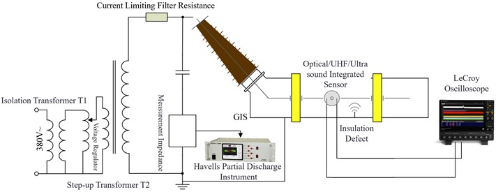
A Gas-Insulated Switchgear (GIS) partial discharge test platform was set up, as shown in the figure. The setup primarily consists of four components: a high-voltage source; a GIS simulation test chamber; a partial discharge detection apparatus; and typical defect models.
As illustrated in Fig. 1, the experimental platform comprises a GIS chamber, an AC voltage regulator, a digital partial discharge meter, an oscilloscope, and sensors. The GIS experimental vessel is filled with 0.5 MPa of SF6 gas. Four types of typical defect models were designed for the experiment: free metal particle discharge, suspended electrode discharge, surface discharge on insulators, and discharge from metallic tips. Each of these models was separately placed into the GIS chamber to conduct partial discharge tests, recording the discharge conditions.
Fig. 1PD detection platform of GIS
PRPD (Phase Resolved Partial Discharge) mapping is a technique used to display the relationship between partial discharge (PD) signals and power supply phase. This type of mapping is particularly useful in Gas-Insulated Switchgear (GIS) because it helps identify different types of partial discharge patterns and can assist in determining whether there are defects within the GIS equipment. In a PRPD map, the horizontal axis typically represents the power supply phase, while the vertical axis indicates the amplitude of the partial discharge. Each point on the map represents a partial discharge detected at a specific power supply phase. Different types of defects lead to distinct PRPD patterns; for example, free metal particles, suspended electrodes, surface defects on insulators, or discharges from metallic tips each exhibit unique characteristics on a PRPD map.
Fig. 2PD spectrum of tip discharge defects
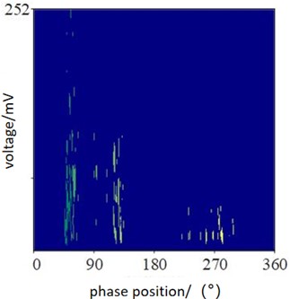
Fig. 2 is a typical PRPD (Phase Resolved Partial Discharge) spectrum indicative of tip discharge characteristics. It displays the variation of partial discharge with respect to the power supply phase. In the figure, the horizontal axis represents the power supply phase (in degrees), and the vertical axis indicates the amplitude of the partial discharge (in microvolts per meter). Each point on the map represents the partial discharge intensity at a specific power supply phase. Extensive research has been devoted to PD pattern recognition methodologies, wherein reference [4] introduces feature extraction techniques grounded in PRPD mapping, tailored specifically for transformer PD pattern discernment. The methodology for extracting features from two-dimensional and three-dimensional partial discharge (PD) patterns hinges upon the tenets of fuzzy entropy expounded in reference [4]. Harnessing the Potential Resolution Phase Display (PRPD), a twelve-dimensional feature realm is established utilizing Linear Predictive Cepstral Coefficients (LPCCs) to meticulously characterize PD signal patterns. Subsequently, to refine this feature terrain, Principal Component Analysis (PCA) is deployed, thereby mapping it onto a two-dimensional space for more streamlined analysis, facilitating the clustering of varied PD categories [5]. Within the realm of PD pattern recognition, efficacious feature extraction stands as a pivotal prerequisite.
Due to the stochastic nature of partial discharges, several machine learning methods for pattern detection and classification have emerged, such as: Support Vector Machines (SVM): Used for classifying GIS partial discharge patterns by determining the optimal hyperplane that maximizes the margin between different discharge types. Decision Trees (DT): Construct hierarchical structures for decision-making, aiding in the identification of conditions leading to specific partial discharge patterns. Random Forests: Combine multiple decision trees to enhance accuracy and robustness, particularly when dealing with noisy datasets. Neural Networks: Utilize deep structures to identify complex PRPD spectrum patterns, improving the accuracy of partial discharge pattern recognition. Genetic Algorithms: Optimize model parameters, such as weights in neural networks, to find the best configuration, thereby enhancing model performance [6-8]. Furthermore, a combination of Recurrent Neural Networks (RNN) and Modified Particle Swarm Optimization (mPSO) is utilized for detecting damage in glass fiber reinforced polymer (GFRP) composite cantilever beams [9-12]. These methodologies are inherently feature-dependent, rendering the caliber of extracted features pivotal to their efficacy in PD identification. Prevailing strategies for feature construction primarily consist of Fourier Transform, Wavelet Transform, Experiential Mode Disassembly, S-Parameter Conversion, and Polar Coordinate Translation [13-16]. Furthermore, to efficaciously distill key PD feature parameters and curtail feature dimensions, Principal Component Analysis (PCA) alongside Autoencoders have been incorporated for GIS-based PD recognition and classification endeavors [17-18].
Still, characteristics display uniqueness; a customized feature ensemble is pertinent exclusively to an individual categorization framework. To overcome this constraint, profound learning techniques have been integrated into GIS pattern discernment and flaw prediction, epitomized by models such as LeNet5, AlexNet, one-dimensional Convolutional Neural Networks (1D-CNN), and LSTM-driven deep recursive neural networks. These methodologies have proven highly applicable [19]-[20]. The LeNet5 model excels in PRPD recognition accuracy. The AlexNet model achieved remarkable outcomes via fusion decision-making, albeit encountering vanishing gradients during training and expanding the model’s storage and computational demands. While 1D-CNN enhances recognition accuracy over 2D convolution, it incurs time increments due to intricate signal handling and fading gradients. LSTM-based deep recurrent networks excel in PRPD pattern analysis but can be influenced by sampling frequencies and feature, potentially leaning excessively on expert intuition. Consequently, novel deep learning frameworks are necessitated to augment recognition precision and real-time fault responsiveness in GIS PD pattern recognition.
Acknowledging the inadequacies in prevailing PD recognition methodologies, this paper introduces a GIS PD pattern recognition strategy that merges Phase-Resolved PD Graph Segmentation (PRPD-Grabcut) with a novel MobileNets Convolutional Neural Network (MCNN) model.
Unlike traditional methods that rely on manually designed features, this paper adopts PRPD-Grabcut technology, using an adaptive threshold image segmentation method to automatically extract key features from PRPD spectra. This approach reduces the dependency on external feature engineering, enhancing the consistency and accuracy of feature extraction.
To address the gradient vanishing problem commonly encountered during the training of traditional deep convolutional neural networks (DCNNs), the MCNN model developed in this paper introduces depthwise separable convolutions and inverted residual structures. These designs not only enhance the model's capability to handle complex tasks but also reduce the number of model parameters and computational complexity, thereby improving training efficiency and recognition accuracy.
Compared to other lightweight neural network models, MCNN demonstrates significant advantages in terms of recognition accuracy, cross-entropy loss, and training time. Particularly in scenarios with limited computational resources, MCNN significantly reduces computational burden and storage space requirements by minimizing model complexity, providing greater flexibility and practicality for real-world applications.
This study proposes a new, efficient, and accurate scheme for GIS partial discharge (PD) pattern recognition, demonstrating superior performance in identifying multiple types of discharges in complex environments. Compared to traditional lightweight networks, the MCNN model shows clear advantages in accuracy, loss reduction, and training speed, filling a technological gap.
Future work will focus on enhancing the model's generalizability and adaptability by expanding the training dataset to recognize a wider variety of PD patterns, thus increasing its applicability in different scenarios; developing a real-time monitoring system version for immediate on-site data processing and fault warnings; optimizing the algorithm for resource-constrained edge devices to support instant data analysis in the field; and exploring the fusion of UHF signals with data from other sensing technologies to obtain more comprehensive fault diagnostic information.
2. Model of this article
2.1. PRPD-Grabcut model
The innovative PRPD-Grabcut technique presented herein is an adaptive threshold-driven image segmentation approach, comprising three successive phases.
Step one: Preprocessing of the Visual Data. Initially, the raw PRPD signals from Ultra-High Frequency (UHF), optical, and ultrasonic domains undergo normalization, ensuring disparate amplitude profiles yield uniform shapes post-normalization. Following normalization, these signals transition into grayscale imagery. Lastly, the normalized grayscale representations undergo division into distinct segments.
Step Two: Integral Image Calculation for Partitioning Purposes. This stage involves the reduction of PRPD representations into binary areas of focus, a common practice in image segmentation methodologies [21]. A square window of dimensions × envelops each central pixel, within which the mean pixel value is computed per the methodology detailed in scholarly work [22]. The integral image at each window's location embodies the pixel summation above and to the left of said window. The crux of PRPD-Grabcut lies in utilizing the mean pixel intensity within the neighborhood block centered at each sliding window's core as the segmentation criterion. Subsequently, a sensitivity threshold (), guided by the noise prevalence in PD monitoring, is established. Spanning the interval [0, 1], this sensitivity parameter gauges the likelihood of pixels being classified as 'object' during segmentation. For windows harboring the target, the instantaneous pixel intensity must fall below t percent of the regional mean.
Step Three: Formation of Diversely Sensitive Segmented Sample Groups and Conversion of PRPD-Grabcut Outputs to Binary Form. Binarization here entails assigning each pixel an RGB value, thereby enriching the description of the image's silhouette and outline.
Step Four: Extraction of Inverted Residual Block (IRB) Characteristics from the segmented spectra of UHF, optical, and ultrasonic partial discharges. The process initiates with Pointwise Convolution expanding the channel breadth, followed by Depthwise Convolution conducting feature extraction through high-dimensional convolution. Lastly, Pointwise Convolution reintroduces dimensionality reduction and channel concatenation, preparing the binary samples for introduction to the recognition model.
2.2. MCNN model
In recent times, Convolutional Neural Networks (CNNs), a paradigmatic deep learning technique, have witnessed rapid advancements and evolved into a potent tool for pattern recognition [23-25]. The feature extraction stratum leverages convolution computations, characterized by sparse interactions, shared parameters, and isomorphism in representation [26]. Sparse interactions permit convolution kernels significantly smaller than the input dimensions, whereas parameter sharing economizes on storage by necessitating only a single set of parameters, thereby imbuing the model with translational equivariance. Moreover, pooling mechanisms maintain a consistent representation despite minor translational shifts in the input. Embracing Deep Convolutional Neural Networks (DCNNs) as classifiers for pattern recognition alleviates the intricacies of manual feature crafting, resolves the underutilization of features, and markedly bolsters diagnostic accuracy and generalizability. Each feature extraction tier initially undergoes a series of convolution operations with diverse kernels. This iterative process within each feature abstraction layer can be encapsulated by Eq. (1):
In this context, ∗ symbolizes the convolution operation; the input , signifying the layer’s constituent elements, is transformed into the output through this process; the bias term is represented by ; the feature map selection is denoted by ; the weights are captured by ; and the kernel function is embodied in . During the convolution process, once the input feature map undergoes convolution computation, it is subsequently channeled through an activation function before being yielded as output. This transformative sequence can be mathematically encapsulated by Eq. (2):
Included herein, signifies the activation function responsible for introducing nonlinearities; ∗ denotes the convolution operation, fundamental to feature extraction; and denote the input and output vectors, respectively, for the layer in question; embodies the coefficient matrix tied to the convolution filter of the matching stratum; and stands for the offset or bias vector. Progressing to the pooling layer, the underlying computational procedure is succinctly encapsulated by Eq. (3), underscoring a dimensionality reduction step that retains essential information while mitigating computational overhead:
Within the fully connected layer, a strategy of weighted summation is employed to analyze the feature maps emanating from the preceding layer. By subjecting these processed features to an activation function, the resultant output feature map is derived, a transformation succinctly encapsulated by Eq. (4). This step essentially fosters direct inter-neuron connectivity, enabling comprehensive integration of learned features for the ultimate classification or regression task:
In this context, the symbol ⋅⋅ denotes the operation of matrix multiplication; the activation function is denoted by ; and represent the initial input and output, respectively; is the weight matrix of the convolution core of the th layer; is the bias vector of the th layer.
The educational objective of a Convolutional Neural Network (CNN) revolves around minimizing the loss function. Should the CNN tackle classification tasks, the loss function employs cross-entropy as its metric, as illustrated in Eq. (5). Conversely, when faced with regression tasks, the mean squared error function assumes the role of the loss function, as exemplified in Eq. (6). This dual approach ensures the network’s versatility across diverse problem domains:
where, is the true value of the -th input; is the predicted value of the -th input; represents the number of samples in the training set; and denotes the model’s parameters, which are the weight vectors.
The MCNN framework constitutes a streamlined deep neural network archetype introduced by Google [27], presenting two iterations: MobileNet-V1 and its successor, MobileNetV2. MobileNet-V1 integrates a depth-wise separable convolution methodology, drastically curtailing the surplus inherent in conventional 3D convolutions. This enhancement not only optimizes latency and shrinks the model footprint but also bolsters the model’s discriminative capability [28]. Building upon the architectural blueprint of MobileNet-V1, MobileNet-V2 integrates a duo of supplementary architectural tenets: the bottleneck and inverted residual structures. These enhancements expedite convergence and stave off degradation phenomena. Given MobileNet-V1’s potential vulnerability to gradient vanishing, this study adopts MobileNet-V2 for the detection and categorization of GIS partial discharge patterns. Fig. 3 illustrates the comprehensive workflow diagram for model training. The process first involves normalizing and converting the original PRPD spectra from UHF, optical, and ultrasonic partial discharge into grayscale, and then segmenting them into smaller samples. Next, integral images of the PRPD samples are calculated, and image segmentation is performed using a sliding window method, where the mean pixel value within the window serves as the segmentation threshold, adjusted by a sensitivity threshold based on the noise level to fine-tune the segmentation sensitivity. Following this, the samples are binarized at different sensitivities to better delineate the shapes and contours in the images. Finally, the segmented spectra undergo feature extraction through an IRB module, utilizing Pointwise and Depthwise convolutions for feature extraction and dimensionality reduction, preparing them for input into the recognition model.
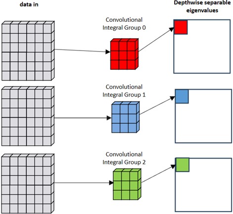
This decomposition can capture features more effectively and improve the parameter utilization and computational efficiency of the model. Depthwise separable convolution first performs depth convolution in the convolution operation, and then performs point-by-point convolution, which can reduce the amount of calculation and model complexity while maintaining the ability to express features.
As shown in Fig. 4, depthwise convolution constitutes a technique that sifts through input channels without inflating their quantity. Suppose an input feature map spans dimensions A×B×C, and the convolution kernel measures ×. When applying convolution to individual feature subsets, the kernel maintains a single channel width. Assuming a kernel ensemble of , each feature subset encounters a solitary P×P kernel [29]. Hence, the arithmetic burden of depth-separable convolution sums up to ABCP², equating to 1/ of Standard convolution’s workload, with equating to . By bypassing channel-wise convolution computations, a substantial diminution in training duration for Multi-Channel Convolutional Neural Networks (MCNN) is attained. This stems from depthwise convolution's approximation to independently harvesting spatial attributes per channel, thereby accelerating the learning trajectory. Such an approach fosters computational efficacy, proving especially advantageous in scenarios entailing voluminous datasets.
Fig. 3Grabcut MCNN training overall flowchart
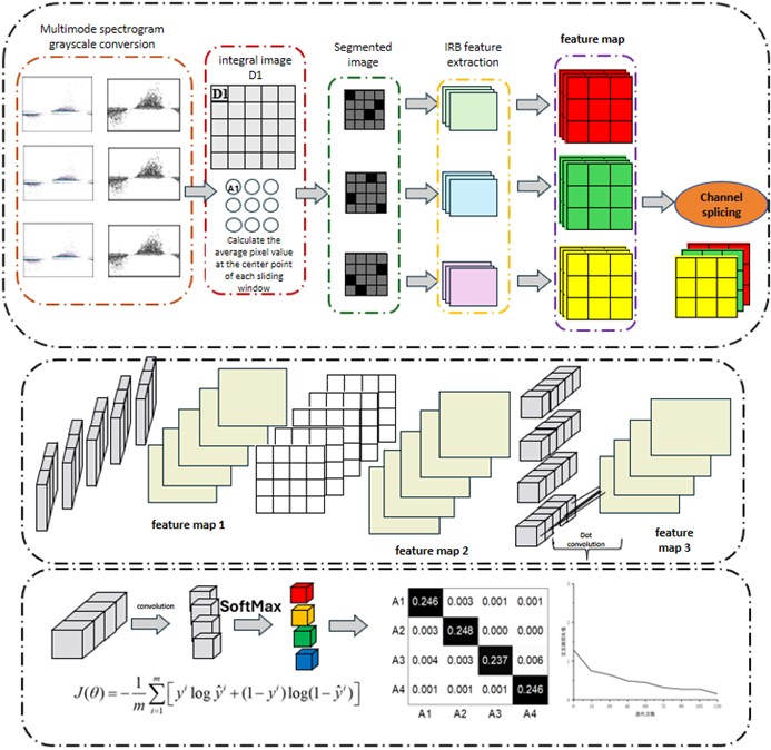
Fig. 4Deep convolutional neural network model
As shown in Fig. 5, pointwise convolution denotes a specialized form of convolution where the kernel size is confined to 1×1. Concretely, given an input feature map of dimensions A×B×C, this operation manifests through executing iterations of 1×1× conventional convolutions, with A×B delineating the map's spatial expanse. Here, signifies the channel count for both the the input characteristic map along with the filtering kernel, while denotes the total convolution kernel quantity. Primarily, pointwise convolution facilitates regulate the output feature map’s channel depth [30]. Computationally, it bears a lighter load, confines to elemental multiplications and accumulations, streamlining calculations. Its prevalence in deep learning circles stems from its versatility in dimensionality modulation, channel expansion, and parameter reduction, thereby augmenting the network’s proficiency in feature extraction.
Fig. 5Point by point convolution operation model
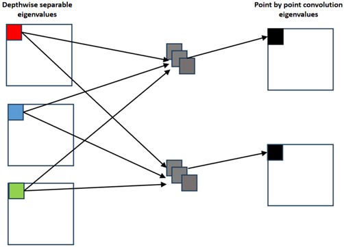
The inverse residual configuration represents a variation on the classic residual architecture. Conventionally, within a standard residual block, we often diminish the feature map's channel count through a bottleneck layer. Conversely, in the inverse residual setup, given that the shortcut linkage attaches to the feature map, necessitating a decrease in channel numbers, this design earns its 'inverse' denomination. In this paper, we propose a new inverse residual model that adopts a different structural design to extract features. First, the number of feature channels is increased through Bottleneck, then a deep convolution layer is used to transform the features, and finally the number of feature channels is reduced through Bottleneck. Different from traditional residual blocks, in the reverse residual operation, we only use deep convolutional layers for nonlinear feature transformation and introduce residual connections between two bottlenecks. This residual connection acts like a traditional residual block, improving convergence and offsetting performance degradation during training. Through the design of this structure, our model has better training effects and performance.
The dimension of the input sample is , and all feature information is included. The characteristics of the sample will be changed into h·x dimensions by the reverse residual structure; ReLU is used to retain the key parts of the special feature and the activation function is discarded in order to prevent the loss of key parts. Finally, bottleneck is used to reduce feature redundancy.
The complete framework of the MobileNet Version 2 design is illustrated within Table 1.
Each horizontal row signifies a singular or plural sequence of operations within an identical network infrastructure. Post y rounds of iterations, every layer partaking in the identical sequence concludes with an equal count of output channels, designated as c. The premier layer sequence initiates with a stride magnitude of q, whereas successive layers adopt a stride length of unity. Spatial convolution kernels uniformly maintain a dimensions of 3×3, while an amplification ratio h is imposed on the incoming features, thoroughly elucidated in Table 1. MobilNet-V2 encompasses an intact convolutional tier equipped with 32 convolutional filters, succeeded by 17 inversed residual bottleneck components. Within this architectural schema, Dropout methodology and Batch Normalization tactics are integrated in the training regimen, alongside the deployment of ReLU6 functioning as the non-linear activation function, which proves more conducive to computations under low-precision constraints. Via these refinements, superfluous elements are efficaciously minimized, thereby curtailing model intricacy without compromising on performance efficacy.
Table 1MobileNet-V2 model architecture
Enter size | Neural networks | ||||
160×160×3 | 2D convolution | – | 28 | 1 | 2 |
80×80×28 | Bottleneck | 1 | 14 | 1 | 1 |
80×80×14 | Bottleneck | 4 | 18 | 2 | 2 |
40×40×18 | Bottleneck | 4 | 28 | 3 | 2 |
20×20×28 | Bottleneck | 4 | 56 | 4 | 2 |
10×10×56 | Bottleneck | 4 | 72 | 3 | 1 |
10×10×72 | Bottleneck | 4 | 180 | 3 | 2 |
5×5×180 | Bottleneck | 4 | 360 | 1 | 1 |
5×5×360 | 1x1 2D convolution | – | 1440 | 1 | 1 |
5×5×1440 | 5x5 average pooling | – | – | 1 | – |
1×1×1440 | 1x1 2D convolution | – | 1000 | – | – |
In MobileNet-V2, we introduced two hyperparameters, the width factor α and the resolution factor to further compress the model. Unlike the width factor value used in MobileNet-V1, which is less than or equal to 1, the width factor value of MobileNet-V2 ranges from 0.31 to 1.35. Such a design enables the width factor to be applied to all layers except the last convolutional layer, which greatly improves the performance of small models. By adjusting the width factor, we can flexibly control the width of the model to balance performance and computational resource consumption. At the same time, introducing a resolution factor can also compress the model to a certain extent, thereby further reducing computational costs. Through these methods, MobileNet-V2 effectively improves the compression ratio of the model while maintaining performance [31-34].
This work harnesses MobileNet-V2 for the purpose of identifying and categorizing patterns characteristic of GIS partial discharges. Initial steps entail the binarization of PRPD-Grabcut samples, a measure aimed at curtailing the model's parameter count. Model training capitalizes on the backpropagation algorithm in conjunction with stochastic gradient descent, fortified by Dropout and Batch Normalization methodologies to bolster training efficacy and expedite the training schedule. At the terminal layer of the model, Softmax serves as the classifier, while one-hot encoding is employed to distinguish among four classes of PD's foundational images. Throughout the model, all activation functions assume the form of ReLU6 functions, enhancing computational efficiency and promoting non-linearity.
3. Experimental analysis
3.1. Analysis of influencing factors of PRPD-Grabcut pattern recognition results
To scrutinize the variables impacting PRPD-Grabcut’s accuracy in pattern discrimination, a dataset comprising 1,250 instances of partial discharge patterns from gas-insulated switchgear was selected. These encompassed scenarios involving free metallic particle discharge, suspended electrode discharge, surface discharge on insulators, and discharges from metallic tips.
PRPD-Grabcut embodies an adaptive threshold-driven image partitioning strategy. As depicted in Figure 6, the relationship between sensitivity settings (0.1, 0.2, 0.3, 0.4, 0.5) and both recognition accuracy and loss metrics is portrayed. Herein, the solid black line traces the trajectory of recognition accuracy, while the intermittent blue line symbolizes the model's cross-entropy loss profile, illustrating how varying sensitivity levels modulate these critical performance indicators.
Illustrated in Fig. 6, the responsiveness parameter significantly influences the outcomes of pattern discernment tasks. Upon configuring the responsiveness at levels of 0.1, 0.2, 0.3, 0.4, and 0.5, the attained recognition precision rates were observed to be 81.27 %, 92.48 %, 97.86 %, 98.28 %, and 97.32 %, respectively, accompanied by cross-entropy loss metrics of 0.71, 0.30, 0.12, 0.02, and 0.08, correspondingly. Notably, when the responsiveness setting reached 0.4, the dataset utilized herein achieved its apex recognition accuracy and concurrently, the most minimized loss magnitude. At this sensitivity setting, the model can more accurately distinguish between target regions and background areas during image segmentation. A higher sensitivity means that more pixels are classified as part of the target, and excessively high sensitivity may introduce too much noise, leading to an increase in false positives, which affects accuracy. Conversely, too low a sensitivity may result in parts of the true target being incorrectly classified as background, thereby reducing accuracy. At a sensitivity of 0.4, the model finds an appropriate balance point, effectively excluding noise interference while maximizing the retention of target information, which helps to improve the model's recognition accuracy. Additionally, the minimization of cross-entropy loss indicates that the model's predicted output is closer to the actual labels, further demonstrating the model's excellent performance at this sensitivity level.
Furthermore, the form and scale of PRPD constitute pivotal elements impacting Grabcut’s efficacy. With the aim of contrasting the repercussions of PRPD visuals exhibiting varied dimensions and resolutions on the exactness of pattern identification, the resolutions used are 10×10, 30×30, 50×50, 70×70, 100×100, 100×150, 100×300, 200 The PRPD images of ×200 and 300×300 are used as input samples of MCNN, and are represented by A1-A9 respectively. The recognition accuracy and cross-entropy values of samples with different resolutions are shown in Fig. 7, in which the black line is the recognition accuracy curve and the blue dotted line is the model cross-entropy loss value.
Fig. 6PD recognition accuracy under different sensitivities
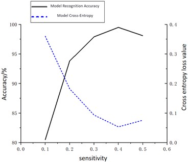
Fig. 7PD recognition accuracy at different resolutions
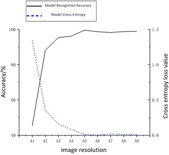
Observations from Fig. 7 reveal that recognition accuracies for resolutions 10×10 and 30×30 remain suboptimal, standing at 43.24 % and 87.96 % correspondingly. However, upon tweaking the sample resolutions to 50×50 and 70×70, a notable upsurge in accuracy is observed, reaching 94.86 % and 95.69 % respectively. Further escalations are marked with resolutions of 100×100, 100×150, 100×300, 200×200, and 300×300, yielding recognition accuracies of 98.24 %, 99.88 %, 99.22 %, 99.67 %, and 99.72 % in that order. Notably, samples rendered at 100×100 resolution outshine others with the pinnacle recognition accuracy coupled with the least loss magnitude.
A lower resolution (such as 10×10 and 30×30) may lead to the loss of important features, thus affecting the model's recognition capability. As the resolution increases (such as to 50×50 and 70×70), more details are retained, allowing the model to better capture these features, hence improving the recognition accuracy. However, an excessively high resolution (such as 300×300) provides more detail but also increases computational complexity and may introduce the risk of overfitting, where the model learns the details of the training data too well and does not generalize well to new data. A resolution of 100×100 retains sufficient detail while avoiding the negative impacts of higher resolutions, thus finding the optimal balance between accuracy and model performance.
3.2. MCNN performance analysis
To ascertain the efficacy of MCNN, the suggested approach is pitted against conventional methodologies (comprising CNN, AlexNet, GoogLeNet, and ResNet) alongside prevalent compact networks (such as SqueezeNet, ShuffleNet, MobileNet, and Xception), as illustrated in Table 2. Regarding the precision of various models, divergent cross-entropy loss scores for these models are depicted in Table 3.
Table 2Different model recognition accuracy
Model | Number of iterations | Accuracy / % |
CNN | 120 | 62.36 |
GoogLeNet | 120 | 73.80 |
Xception | 120 | 62.12 |
AlexNet | 120 | 71.39 |
ResNet | 120 | 80.12 |
SqueezeNet | 120 | 75.41 |
SuffleNet | 120 | 76.98 |
MobileNet | 120 | 69.84 |
MCNN | 120 | 91.46 |
Table 2 illustrates that MCNN surpasses alternative neural networks in terms of recognition precision. By the 120th cycle, the educational preciseness for CNN stood at 62.36 %, for GoogLeNet it reached 73.80 %, whereas MCNN achieved an educational preciseness of 91.46 %.
This result indicates that MCNN possesses stronger learning capabilities and higher recognition accuracy. The primary reasons for this phenomenon are the more effective feature extraction methods and optimization strategies adopted by MCNN, such as depthwise separable convolutions and inverted residual structures. These techniques not only reduce the complexity and computational burden of the model but also enhance the training efficiency and recognition accuracy. Depthwise separable convolutions decrease the computational load by performing depthwise convolution followed by pointwise convolution, maintaining the expressive power of features. Inverted residual structures help alleviate the vanishing gradient problem, improving the stability of model training. These mechanisms work together, enabling MCNN to converge faster during the training process and achieve better performance within the same number of training cycles.
Table 3Cross-entropy loss of different models
Model | Initial cross entropy loss value | Terminal cross entropy loss value |
CNN | 2.8674 | 0.9468 |
GoogLeNet | 2.3247 | 0.7245 |
Xception | 2.4587 | 0.5621 |
AlexNet | 1.8756 | 0.7213 |
ResNet | 1.5879 | 0.6541 |
SqueezeNet | 1.3684 | 0.5679 |
SuffleNet | 1.5214 | 0.5395 |
MobileNet | 1.6847 | 0.6595 |
MCNN | 1.142 | 0.1725 |
According to Table 3, MCNN demonstrates a notably diminished loss magnitude in contrast with other network architectures. Commencing with the highest initial loss figure of 2.9042, CNN contrasts with MCNN, which initiates at the lowest loss level of 1.142. Upon reaching 120 iterative cycles, CNN's concluding loss magnitude peaks at 0.9468, whereas MCNN maintains the least loss value at 0.1725. This evidences that MCNN excels in both precision for PD recognition and the velocity of convergence, outperforming both conventional neural frameworks and currently established compact network models.
The primary reasons for this result are due to the depthwise separable convolutions and the inverted residual structures. Depthwise separable convolutions break down the convolution operation into two separate steps – depthwise convolution and pointwise convolution – effectively reducing the demand for computational resources while maintaining the ability to extract features. Inverted residual structures help address the issue of vanishing gradients, ensuring stability during the training process, which in turn accelerates the convergence speed of the model. These technologies work together to allow MCNN to achieve a lower loss value from the early stages of training and to maintain a low loss as training progresses, thereby achieving efficient and accurate PD recognition.
3.3. PRPD-Grabcut-MCNN performance analysis
In order to verify the performance of PRPD-Grabcut-MCNN, the accuracy and model training time of each network model were compared, as shown in Figs. 8-9.
Fig. 8PD recognition accuracy under different network models
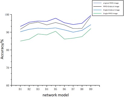
Fig. 9Model training time under different network models
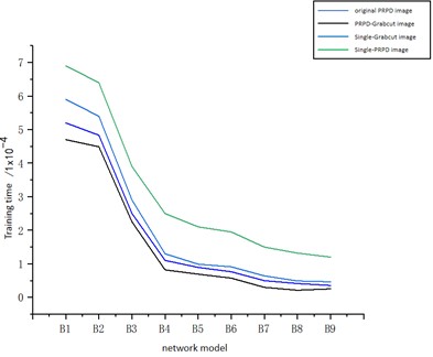
In Figs. 8 and 9, B1 to B9 represent CNN, GoogLeNet, Xception, AlexNet, ResNet, SqueezeNet, ShuffleNet, MobileNet, and the model proposed in this paper, respectively. Fig. 7 shows the recognition accuracy of each model when the inputs are multi-source original PRPD patterns, multi-source PRPD patterns processed by PRPD-Grabcut, single-source original PRPD patterns, and single-source PRPD patterns processed by PRPD-Grabcut. Fig. 8 illustrates the loss function of each model corresponding to the same sets of inputs. As Figs. 7-8 illustrate, the identification precision of samples processed via PRPD-Grabcut is notably superior to that of unmodified PRPD samples. With respect to training duration, the PRPD-Grabcut methodology curtails the time required for network model training in comparison to its unprocessed PRPD image counterparts. Moreover, irrespective of whether a solitary input comprises the pristine PRPD image or an image subjected to the Grabcut-PRPD process, the resultant training efficiency pales in contrast to scenarios incorporating multi-modal inputs, highlighting the inferiority of single-input methodologies in this context.
Regarding PRPD-Grabcut samples, the recognition accuracies of CNN, GoogLeNet, AlexNet, and ResNet stand at 91.18 %, 94.46 %, 96.35 %, and 96.58 % respectively. Remarkably, MCNN achieves a 99.91 % recognition accuracy, surpassing CNN by 8.73 %. Relative to unprocessed PRPD samples, the employment of PRPD-Grabcut samples elevates MobileNet’s recognition accuracy by 1.05 % and ResNet’s by 3.33 %.
Lightweight neural networks notably trim down training durations compared to their conventional counterparts. The MCNN put forth in this study successfully realizes model lightweighting. When applied to PRPD-Grabcut samples, training durations for CNN, GoogLeNet, AlexNet, and ResNet amount to 48,523, 45,342, 23,024, and 8,325 seconds, respectively. Conversely, Xception, SqueezeNet, ShuffleNet, and MobileNet clock in at 7,464, 5,128, 4,435, and 4,115 seconds. MCNN, with a training time of 2,543 seconds, demands 16,24 seconds less than MobileNet alone. Consequently, the MCNN framework, grounded in PRPD-Grabcut, dramatically curtails the model’s computational load, concurrently boosting PD recognition accuracy and abbreviating network training periods. In juxtaposition with an array of established lightweight neural networks, MCNN distinguishes itself through superior recognition accuracy and abbreviated training intervals.
4. Conclusions
This paper adopts PRPD-Grabcut technology, using an adaptive threshold image segmentation method to automatically extract key features from PRPD spectra. This approach reduces the dependency on external feature engineering, enhancing the consistency and accuracy of feature extraction. To address the gradient vanishing problem commonly encountered during the training of traditional deep convolutional neural networks (DCNNs), the MCNN model developed in this paper introduces depthwise separable convolutions and inverted residual structures. These designs not only enhance the model's capability to handle complex tasks but also reduce the number of model parameters and computational complexity, thereby improving training efficiency and recognition accuracy. Compared to other lightweight neural network models, MCNN demonstrates significant advantages in terms of recognition accuracy, cross-entropy loss, and training time. Particularly in scenarios with limited computational resources, MCNN significantly reduces computational burden and storage space requirements by minimizing model complexity, providing greater flexibility and practicality for real-world applications.
References
-
S. Zheng and S. Wu, “Detection study on propagation characteristics of partial discharge optical signal in GIS,” IEEE Transactions on Instrumentation and Measurement, Vol. 70, pp. 1–12, Jan. 2021, https://doi.org/10.1109/tim.2021.3106117
-
Y. Yuan, S. Ma, J. Wu, B. Jia, W. Li, and X. Luo, “Frequency feature learning from vibration information of GIS for mechanical fault detection,” Sensors, Vol. 19, No. 8, p. 1949, Apr. 2019, https://doi.org/10.3390/s19081949
-
J. Li and A. Wang, “Intelligent defect diagnosis of GIS basin insulator via multi-source ultrasonic fusion,” Nondestructive Testing and Evaluation, Vol. 39, No. 6, pp. 1454–1466, Aug. 2024, https://doi.org/10.1080/10589759.2023.2273999
-
K. Firuzi, M. Vakilian, B. T. Phung, and T. R. Blackburn, “Partial discharges pattern recognition of transformer defect model by LBP and HOG features,” IEEE Transactions on Power Delivery, Vol. 34, No. 2, pp. 542–550, Apr. 2019, https://doi.org/10.1109/tpwrd.2018.2872820
-
C.-K. Chang, B. K. Boyanapalli, and R.-N. Wu, “Application of fuzzy entropy to improve feature selection for defect recognition using support vector machine in high voltage cable joints,” IEEE Transactions on Dielectrics and Electrical Insulation, Vol. 27, No. 6, pp. 2147–2155, Dec. 2020, https://doi.org/10.1109/tdei.2020.009055
-
Q. Khan, S. S. Refaat, H. Abu-Rub, and H. A. Toliyat, “Partial discharge detection and diagnosis in gas insulated switchgear: State of the art,” IEEE Electrical Insulation Magazine, Vol. 35, No. 4, pp. 16–33, Jul. 2019, https://doi.org/10.1109/mei.2019.8735667
-
R. Umamaheswari and R. Sarathi, “Identification of partial discharges in gas-insulated switchgear by ultra-high-frequency technique and classification by adopting multi-class support vector machines,” Electric Power Components and Systems, Vol. 39, No. 14, pp. 1577–1595, Oct. 2011, https://doi.org/10.1080/15325008.2011.596506
-
M. Wu, H. Cao, J. Cao, H.-L. Nguyen, J. B. Gomes, and S. P. Krishnaswamy, “An overview of state-of-the-art partial discharge analysis techniques for condition monitoring,” IEEE Electrical Insulation Magazine, Vol. 31, No. 6, pp. 22–35, Nov. 2015, https://doi.org/10.1109/mei.2015.7303259
-
B. B. Bal, S. P. Parida, and P. C. Jena, “Damage assessment of beam structure using dynamic parameters,” in Lecture Notes in Mechanical Engineering, Singapore: Springer Singapore, 2020, pp. 175–183, https://doi.org/10.1007/978-981-15-2696-1_17
-
S. Sahoo, S. P. Parida, and P. C. Jena, “Dynamic response of a laminated hybrid composite cantilever beam with multiple cracks and moving mass,” Structural Engineering and Mechanics, Vol. 87, No. 6, pp. 529–540, Sep. 2023, https://doi.org/10.12989/sem.2023.87.6.529
-
S. P. Parida and P. C. Jena, “Dynamic analysis of cracked FGM cantilever beam,” in Lecture Notes in Mechanical Engineering, Singapore: Springer Singapore, 2020, pp. 339–347, https://doi.org/10.1007/978-981-15-2696-1_33
-
S. P. Parida, S. Sahoo, and P. C. Jena, “Prediction of multiple transverse cracks in a composite beam using hybrid RNN-mPSO technique,” Proceedings of the Institution of Mechanical Engineers, Part C: Journal of Mechanical Engineering Science, Vol. 238, No. 16, pp. 7977–7986, Mar. 2024, https://doi.org/10.1177/09544062241239415
-
W. Pan et al., “Material plastic properties characterization using a generic algorithm and finite element method modelling of the plane-strain small punch test,” in SPT Conference, 2010.
-
Z. Ren, M. Dong, M. Ren, H.-B. Zhou, and J. Miao, “The study of partial discharge in GIS under impulse voltage based on time-frequency analysis,” in 2012 IEEE International Conference on Condition Monitoring and Diagnosis (CMD), Vol. 38, pp. 694–697, Sep. 2012, https://doi.org/10.1109/cmd.2012.6416240
-
D. Dai, X. Wang, J. Long, M. Tian, G. Zhu, and J. Zhang, “Feature extraction of GIS partial discharge signal based on S‐transform and singular value decomposition,” IET Science, Measurement and Technology, Vol. 11, No. 2, pp. 186–193, Mar. 2017, https://doi.org/10.1049/iet-smt.2016.0255
-
J. Xue, X.-L. Zhang, W.-D. Qi, G.-Q. Huang, B. Niu, and J. Wang, “Research on a method for GIS partial discharge pattern recognition based on polar coordinate map,” in 2016 IEEE International Conference on High Voltage Engineering and Application (ICHVE), Vol. 27, pp. 1–4, Sep. 2016, https://doi.org/10.1109/ichve.2016.7800595
-
Y. Wang, J. Yan, Z. Yang, Z. Qi, J. Wang, and Y. Geng, “A novel domain adversarial graph convolutional network for insulation defect diagnosis in gas-insulated substations,” IEEE Transactions on Power Delivery, Vol. 38, No. 1, pp. 442–452, Feb. 2023, https://doi.org/10.1109/tpwrd.2022.3190938
-
X. Peng et al., “A convolutional neural network-based deep learning methodology for recognition of partial discharge patterns from high-voltage cables,” IEEE Transactions on Power Delivery, Vol. 34, No. 4, pp. 1460–1469, Aug. 2019, https://doi.org/10.1109/tpwrd.2019.2906086
-
S. Li et al., “Partial discharge detection and defect location method in GIS cable terminal,” Energies, Vol. 16, No. 1, p. 413, Dec. 2022, https://doi.org/10.3390/en16010413
-
J. Zheng, Z. Chen, Q. Wang, H. Qiang, and W. Xu, “GIS partial discharge pattern recognition based on time-frequency features and improved convolutional neural network,” Energies, Vol. 15, No. 19, p. 7372, Oct. 2022, https://doi.org/10.3390/en15197372
-
Y. Fu, J. Fan, S. Xing, Z. Wang, F. Jing, and M. Tan, “Image segmentation of cabin assembly scene based on improved RGB-D Mask R-CNN,” IEEE Transactions on Instrumentation and Measurement, Vol. 71, pp. 1–12, Jan. 2022, https://doi.org/10.1109/tim.2022.3145388
-
Y. Chai et al., “Texture-sensitive superpixeling and adaptive thresholding for effective segmentation of sea ice floes in high-resolution optical images,” IEEE Journal of Selected Topics in Applied Earth Observations and Remote Sensing, Vol. 14, pp. 577–586, Jan. 2021, https://doi.org/10.1109/jstars.2020.3040614
-
S. Hershey et al., “CNN architectures for large-scale audio classification,” in IEEE International Conference on Acoustics, Speech and Signal Processing (ICASSP), pp. 131–135, Mar. 2017, https://doi.org/10.1109/icassp.2017.7952132
-
S. Ji, W. Xu, M. Yang, and K. Yu, “3D convolutional neural networks for human action recognition,” IEEE Transactions on Pattern Analysis and Machine Intelligence, Vol. 35, No. 1, pp. 221–231, Jan. 2013, https://doi.org/10.1109/tpami.2012.59
-
D. Scherer, A. Müller, and S. Behnke, “Evaluation of pooling operations in convolutional architectures for object recognition,” in Lecture Notes in Computer Science, pp. 92–101, Jan. 2010, https://doi.org/10.1007/978-3-642-15825-4_10
-
M. Belkin and P. Niyogi, “Laplacian eigenmaps for dimensionality reduction and data representation,” Neural Computation, Vol. 15, No. 6, pp. 1373–1396, Jun. 2003, https://doi.org/10.1162/089976603321780317
-
A. G. Howard et al., “MobileNets: Efficient convolutional neural networks for mobile vision applications,” ArXiv, abs/1704.04861, Vol. abs/1704.04861, 2017.
-
S. Kornblith, J. Shlens, and Q. V. Le, “Do better imagenet models transfer better?,” in IEEE/CVF Conference on Computer Vision and Pattern Recognition (CVPR), pp. 2656–2666, Jun. 2019, https://doi.org/10.1109/cvpr.2019.00277
-
K. He, X. Zhang, S. Ren, and J. Sun, “Deep residual learning for image recognition,” in 2016 IEEE Conference on Computer Vision and Pattern Recognition (CVPR), pp. 770–778, Jun. 2016, https://doi.org/10.1109/cvpr.2016.90
-
Q. Kang, H. Zhao, D. Yang, H. S. Ahmed, and J. Ma, “Lightweight convolutional neural network for vehicle recognition in thermal infrared images,” Infrared Physics and Technology, Vol. 104, p. 103120, Jan. 2020, https://doi.org/10.1016/j.infrared.2019.103120
-
M. Tan et al., “MnasNet: platform-aware neural architecture search for mobile,” in IEEE/CVF Conference on Computer Vision and Pattern Recognition (CVPR), pp. 2820–2828, Jun. 2019, https://doi.org/10.1109/cvpr.2019.00293
-
S. Han et al., “Partial discharge pattern recognition in GIS based on EFPI sensor,” Electric Power Engineering Technology, Vol. 41, No. 1, pp. 149–155, 2022, https://doi.org/10.12158/j.2096-3203.2022.01.020
-
Liao Jingwen et al., “GIS vibration signal denoising and mechanical defect identification based on CycleGAN and CNN,” (in Chinese), Electric Power Engineering Technology, Vol. 42, No. 5, pp. 37–45, 2023, https://doi.org/10.12158/j.2096-3203.2023.05.005
-
X. Jiang et al., “Digitalization transformation of power transmission and transformation under the background of new power system,” High Voltage Engineering, Vol. 48, No. 1, pp. 1–10, 2022, https://doi.org/10.13336/j.1003-6520.hve.20211649
About this article
Project Supported by the Science and Technology Project of State Grid Corporation of China (5500-202218132A-1-1-ZN).
The datasets generated during and/or analyzed during the current study are available from the corresponding author on reasonable request.
Zhen Wang mathematical model and the simulation techniques. Hui Fu spelling and grammar checking as well as virtual validation. Chengbo Hu data interpretation and paper revision. Ziquan Liu data collection and data sorting. Yujie Li writing – original draft preparation. Weihao Sun experimental validation.
The authors declare that they have no conflict of interest.
