Abstract
Hyperspectral images (HSIs) contain rich spectral information characteristics. Different spectral information can be used to classify different types of ground objects. However, the classification effect is mainly determined by the quality of spectral characteristic information and the performance of the classifier. This paper explores the use of two-dimensional empirical mode decomposition (2D-EMD) to first feature extraction of HSIs, then uses 2D-EMD to carry out adaptive decomposition of each band of hyperspectral data, and optimally extract the features of the sub-band obtained by decomposition. Then, the optimized features are classified in the support vector machine (SVM) recognition classifier optimized by grey wolf optimization (GWO) algorithm to further improve the effect of network recognition and classification. The simulation results show that this scheme can further improve the recognition results of different ground objects in HSIs.
1. Introduction
The development of high-resolution satellite imaging sensors has enhanced the collection of remote sensing data and provided a cost-effective method to capture large amounts of feature information. Hyperspectral images (HSIs) contain rich one-dimensional (1D) spectral dimension information and two-dimensional (2D) spatial domain feature information [1]. By extracting useful feature information components of HSIs, different features can be classified, unmixed, denoised and compressed. HSIs technology has been widely used in agricultural resource management, marine resource monitoring, mineral exploitation and other aspects [2], [3].
HSIs acquired by spaceborne or airborne sensors usually record hundreds of spectral wavelengths per pixel in the image, which opens up new perspectives for many applications in remote sensing. Since subtle differences in ground cover can be picked up by different spectral features, HSIs is a technique well suited to distinguishing materials of interest. While the rich spectral features can provide useful information for data analysis, the high dimension of HSIs data also presents some new challenges.
In the application of HSIs classification, one of the main factors affecting classification is to consider suitable feature extraction methods. However, the types of satellite images provided by different imaging sensors vary greatly due to different spatial and spectral resolution, which makes the feature extraction process more complicated. According to some literature studies, 2D spatial domain feature extraction is more effective than 1D feature extraction [4], [5]. Literature [6] proposes an empirical mode decomposition (EMD) method to extract features from hyperspectral remote sensing data sets, and also compares the recognition results of 2D decomposition scheme and 1D decomposition method. The results show that the 2D scheme is more effective than the 1D scheme. In addition, according to the characteristics of two-dimensional empirical mode decomposition (2D-EMD), each band image of HSIs can be decomposed into a sub-band image from high frequency to low frequency. The high frequency of image contains the high frequency detail features of the original image, such as edges, textures and contours. The low frequency sub-band image contains the low frequency division of the original image. The results show that the low frequency component in the sub-band image is better for classification.
Spectral classification of HSIs takes pixel vector (spectral feature) as the only feature. In pixel-by-pixel classification (spectral classification), we need to classify the extracted feature information, and the selection of classifier is another major factor affecting the classification effect. Support vector machine (SVM) is an effective HSIs classification method, but the problem of parameter allocation poses a challenge to the accurate classification of HSIs [7], [8]. Some parameter optimization algorithms can improve the performance of SVM network. For example, in literature [9], [10], the Genetic Algorithm (GA) method is used to optimize and then classify the recognition network. In literature [11], [12], particle swarm optimization (PSO) was applied to the classification of HSIs. Inspired by similar ideas, this paper proposes to use grey wolf optimization (GWO) to further improve the SVM network recognition performance of feature samples obtained from 2D-EMD, so as to provide better classification effect for HSIs classification. In this paper, the data mining of HSIs data is studied. After feature extraction of HSIs, the feasibility of the scheme is evaluated by using the classification effect of different ground objects [13-15]. The feature extraction and classifier network, two main factors that affect the classification effect, are comprehensively considered and analyzed [7], [16].
The rest of the article is organized as follows. In Section 2, the 2D-EMD feature extraction method and classifier network SVM are briefly described, and the optimization algorithm GWO is introduced. Section 3 is the experimental process and results analysis. Section 4 is the conclusion of the paper.
2. Methodology
2.1. 2D-EMD
The 2D-EMD is a 2D extended version of 1D-EMD. The EMD can decompose the nonlinear non-stationary signal into several natural mode components (IMFs). The first decomposed component is the high frequency component of the original signal, and the last screened natural mode component is the low frequency component of the original signal. This method has good adaptive characteristics. According to this characteristic, the method is often used in different fields of signal denoising, feature extraction and so on. The process of obtaining IMF functions is called screening, and it is an iterative process. Typical threshold difference (SD) ranges from 0.2 to 0.3.
2D extension form is mainly used in image processing. Image decomposition by 2D-EMD is a scale decomposition process from small to large. Firstly, the edge details of the image are extracted, and then the smoothing region is gradually screened. 2D-EMD can set stop criteria and boundary conditions without setting basis function, and can easily decompose images from small to large scale. The last pattern component to be filtered is also known as the remainder. After screening, surface information of different scales can be further extracted. The decomposition component can be obtained through the decomposition process of narrowband filter, so there is a strong correlation between pixel components, which can be regarded as a complete process of image fusion.
Assuming that HSIs is represented as R{W×H×K}, W is the width of the spatial band, H is the height of the spatial band, and K is the total number of bands in the data set. each band of HSI can be represented by the following expression after being decomposed by 2D-EMD:
where B(i,j) represents the spatial position of each band of HSI data. The k is the kth band image (k=1,2,⋯,K). The n is the number of natural IMFs obtained by decomposition of each band of HSI data (n=1,2,⋯,N). Res represents the residual component obtained by decomposition. In some applications you can think of this component as the last proper IMF component.
2.2. GWO
The GWO Algorithm is a new meta heuristic optimization algorithm proposed by Mirjalili S et al., which has good convergence speed and optimization accuracy and has been widely applied in multiple research fields [17].
The GWO algorithm simulates the hierarchical leadership mechanism of the social organization of the grey wolf population, which involves the collective hunting behavior from searching for prey, surrounding prey to hunting, and continuously iteratively optimizing to obtain the optimal solution location. The GWO algorithm simulates the behavior of wolf packs in three main steps: surround, hunt, and attack. The specific process is as follows: During the optimization process, the population will search for the best hunting route by surrounding the prey. The target position and optimal population position during the orbit stage can be determined by Eqs. (2) and (3):
where the t is the current number of iterations, A, C and D are the coefficient vectors, Xp(t)Xp(t) is the target optimal solution vector (the location of prey), X(t) is the current position vector of a search individual, and X(t+1) is the next moving direction vector. A and C can be represented as follows:
where the M is the maximum number of iterations, a linearly decreases from 2 to 0 as the number of iterations t increases, r1r1and r2 are the random vectors between [0,1]. According to Eqs. (5-6), the location of the points around the optimal solution can be searched by adjusting the size of the coefficient vectors of A and C to ensure the local optimization ability of the algorithm. r1r1 and r2r2 are random numbers between [0, 1], so the optimization population can find all the paths of the attacking target, while ensuring the global search ability of the algorithm.
When hunting and attacking prey, ω moves in the next step according to the signals sent by α, β and δ to judge whether it is close to the target or far away. The specific process can be expressed by Eq. (7-9):
where DαDα,DβDβ and Dδ are the direction vectors between α, β, δ and ω, respectively. The X1X1, X2X2 and X3X3 are respectively α, β and δ to determine the direction vector of ω next move.
2.3. GWO-SVM
When network identification is carried out on sample data, network parameters should be selected appropriately. Here we select radial basis kernel function which is widely used for classification training. In network training, the penalty factor parameter c and the radial basis kernel function’s gamma parameter are two very important parameters that affect the classification results.
In this paper, the GWO algorithm is applied to different training and test samples of hyperspectral data sets, and the SVM network classifier performs parameter optimization, which can further improve the classification results of SVM and further improve the separable performance of the features extracted from 2D-EMD.
3. Experimental analysis
The introduction of Section 3 mainly includes three parts. Section 3.1 mainly introduces the whole experimental procedure. Section 3.2 mainly introduces the characteristics of the data set used in the experiment. In Section 3.3, the experimental results are shown in graphs and tables, and the experimental results and phenomena are analyzed in detail.
3.1. Experimental procedure
The whole process of the experiment mainly includes six main steps. The experimental flow scheme is shown in Fig. 1.
Fig. 1Flow chart of experimental scheme
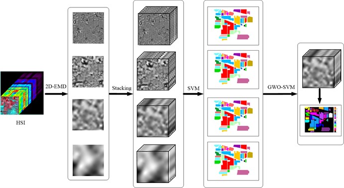
The first step of the experiment is to select the object of analysis, that is, to determine the application scenario of the research. Preprocess the selected data set and select the band data we need to analyze, because some of the bands have a lot of noise effect. In step 2, perform 2D-EMD decomposition for each band of the data set to obtain sub-band images of different frequency bands. In step 3, the sub-band image obtained from each band decomposition is reconstructed, and a new cube feature data set is obtained for each sub-band image. In step 4, conduct SVM classification on the obtained new cube data set, and compare the classification effect of different frequency bands respectively. In step 5, select the band cube data set with the best classification effect. In step 6, introduce the optimal frequency band cube data set into the network optimized by GWO-SVM for classification operation.
Thus, further improve the analysis effect of different types of ground objects. The two main factors that affect the recognition and classification results, feature extraction and classifier, are considered.
3.2. Datasets
3.2.1. Datasets introduction
The data set used in the experiment consists of three types of scenarios. The selected HSIs data is widely used as the main validation data set for studying HSIs classification. Experimental simulation data download link address: https://www.ehu.eus/ccwintco/index.php?title=Hyperspectral_Remote_Sensing_Scenes.
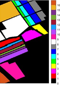
The first Indian Pine scene was collected by AVIRIS sensor at Indian Pine Proving ground in northwest Indiana. It consisted of 145 × 145 pixels and 224 spectral reflection bands. After removing noise bands, 200 bands were left for further analysis. The Indian Pine dataset contains a total of 16 feature categories. Detailed references to the data are shown in Table 1 and Fig. 2.
Fig. 2Indian Pine dataset
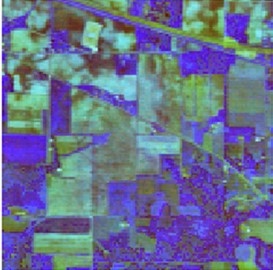
a) False composite image
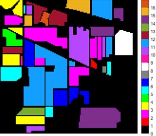
b) Ground truth map
Table 1Number of samples (NoS) for each class of the Indian Pine dataset
Class | Color | Class name | NoS |
1 | Alfalfa | 46 | |
2 | Corn-notill | 1428 | |
3 | Corn-mintill | 830 | |
4 | Corn | 237 | |
5 | Grass-pasture | 483 | |
6 | Grass-trees | 730 | |
7 | Grass-pasture-mowed | 28 | |
8 | Hay-windrowed | 478 | |
9 | Oats | 20 | |
10 | Soybean-notill | 972 | |
11 | Soybean-mintill | 2455 | |
12 | Soybean-clean | 593 | |
13 | Wheat | 205 | |
14 | Woods | 1265 | |
15 | Buildings-Grass-Trees-Drives | 386 | |
16 | Stone-Steel-Towers | 93 |
The second Salinas scene data was captured by a 224-band AVIRIS sensor over the Salinas Valley in California and features high spatial resolution. After removing the noise bands, 204 bands were left for further analysis. The space size of each band is 512×217. The Salinas dataset contains a total of 16 feature categories. Detailed references to the data are shown in Table 2 and Fig. 3.
Table 2Number of samples (NoS) for each class of the Salinas dataset
Class | Color | Class name | NoS |
1 | Brocoli_green_weeds_1 | 2009 | |
2 | Brocoli_green_weeds_2 | 3726 | |
3 | Fallow | 1976 | |
4 | Fallow_rough_plow | 1394 | |
5 | Fallow_smooth | 2678 | |
6 | Stubble | 3959 | |
7 | Celery | 3579 | |
8 | Grapes_untrained | 11271 | |
9 | Soil_vinyard_develop | 6203 | |
10 | Corn_senesced_green_weeds | 3278 | |
11 | Lettuce_romaine_4wk | 1068 | |
12 | Lettuce_romaine_5wk | 1927 | |
13 | Lettuce_romaine_6wk | 916 | |
14 | Lettuce_romaine_7wk | 1070 | |
15 | Vinyard_untrained | 7268 | |
16 | Vinyard_vertical_trellis | 1807 |
Fig. 3Salinas dataset
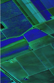
a) False composite image
b) Ground truth map
The third scenario data is from the Kennedy Space Center (KSC). The KSC dataset was acquired by NASA's Airborne Visible/Infrared Imaging Spectrometer (AVIRIS) over the Kennedy Space Center in Florida. AVIRIS obtained data for 224 bands, which were analyzed using 176 bands after removing water absorption and low signal-to-noise ratio bands. The space size of each band is 512×614. Recognition of land cover in this environment is difficult due to the similar spectral characteristics of some vegetation types. For classification purposes, 13 categories were defined for the site, representing the various land cover types occurring in the environment. Detailed references to the data are shown in Table 3 and Fig. 4.
Table 3Number of samples (NoS) for each class of the KSC dataset
Class | Color | Class name | NoS |
1 | Scrub | 761 | |
2 | Willow swamp | 243 | |
3 | Cabbage palm hammock | 256 | |
4 | Cabbage palm/oak hammock | 252 | |
5 | Slash pine | 161 | |
6 | Oak/broadleaf hammock | 229 | |
7 | Hardwood swamp | 105 | |
8 | Graminoid marsh | 431 | |
9 | Spartina marsh | 520 | |
10 | Cattail marsh | 404 | |
11 | Salt marsh | 419 | |
12 | Mud flats | 503 | |
13 | Wate | 927 |
Fig. 4KSC dataset
a) False composite image
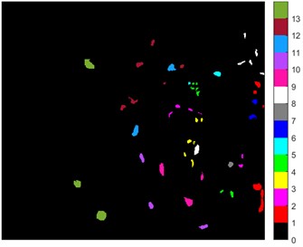
b) Ground truth map
3.2.2. Spectral characteristics of the datasets
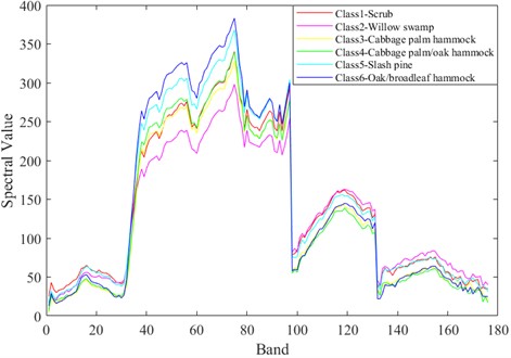
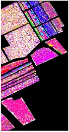
In Fig. 5-7 respectively shows the spectral values of the three data sets in different categories of ground objects. The abscissa in the figure represents the number of bands and the ordinate represents the spectral value.
The Indian Pine dataset was preprocessed to contain 200 spectral bands for analysis. As can be seen from Fig. 5, spectral curves of the first 6 types of ground objects have different spectral values in different bands. In the first 80 bands, the spectral values of different ground objects are highly distinguishable. The Salinas dataset, after being preprocessed, contains 204 spectral bands for analysis. As can be seen from Fig. 6, in the first 100 bands, the spectral values of different ground objects are highly differentiated. In Fig. 7, KSC contains 176 bands after pretreatment for analysis. It can be clearly seen in Fig. 7 that the spectral values of the first 6 different types of ground objects are highly distinguishable when the band interval is between 40 and 100. Different features of spectral curves can be used to classify different types of ground objects. The spectral values of Indian Pine and Salinas data sets are much larger than those of KSC. However, it can also be seen from the spectral curves of the two types of data that the spectral curves overlap, which often leads to low feature differentiation of different categories of ground objects, which will affect the effect of classification. Therefore, in the classification, it is necessary to carry out effective feature extraction for spectral features, and also put forward higher requirements for classifier network.
Fig. 5Spectral values of ground objects from categories 1 to 6 in the Indian Pine dataset
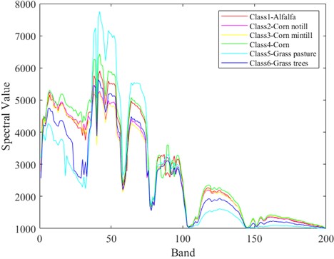
Fig. 6Spectral values of ground objects from categories 1 to 6 in the Salinas dataset
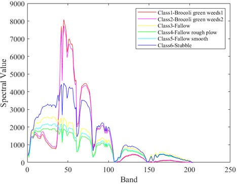
Fig. 7Spectral values of ground objects from categories 1 to 6 in the KSC dataset
4. Experimental result
Table 4 shows the comparison of recognition results of three sets of scene data under different natural pattern components. Here, the training samples and tests are directly imported into the SVM network for classification, and radial basis kernel functions with good performance are adopted. In order to avoid randomness brought by experiments, we take the mean and standard deviation of 10 experiments as statistical results. Here, the evaluation indexes OA and Kappa are adopted for measurement [7, 14-16]. Raw is the benchmark reference value for our comparison. It can be seen from Table 4 that the reference value of the second group of Salinas data set is higher, indicating that the difficulty of feature extraction is less, and the spectral curve features are more conducive to classification. The first Indian Pine dataset had the lowest reference value, indicating the greatest difficulty in feature extraction. According to the classification results of the three groups of data, the effect of the lower component is the best, indicating that the low frequency component is more conducive to classification.
Table 4Classification results of three data sets in different IMFs
Feature | Evaluation | Indian Pine | Salinas | KSC |
Raw | OA | 73.50±1.05 | 89.94±0.40 | 79.53±1.05 |
Kappa×100 | 70.40±1.89 | 88.77±0.46 | 77.15±1.18 | |
IMF1 | OA | 53.65±0.72 | 39.50±0.84 | 48.03±3.20 |
Kappa×100 | 45.61±1.00 | 91.09±1.18 | 41.52±3.33 | |
IMF2 | OA | 86.54±0.86 | 59.94±1.09 | 57.62±3.24 |
Kappa×100 | 84.50±0.99 | 54.71±1.26 | 52.10±3.83 | |
IMF3 | OA | 95.06±0.48 | 92.23±1.08 | 74.21±2.23 |
Kappa×100 | 94.36±0.55 | 91.31±1.22 | 70.90±2.63 | |
IMF4 | OA | 93.63±1.03 | 97.01±0.67 | 81.74±2.69 |
Kappa×100 | 92.74±1.17 | 96.67±0.75 | 79.50±3.03 |
In the first part of the introduction, we mentioned that there are two key factors affecting classification, the first is the choice of feature extraction scheme, and the other is the quality of classifier. According to these two characteristics, we select the best mode component of the three data sets for the second optimization. Kernel function parameters and penalty factor parameters in SVM training network were optimized, and GWO algorithm was used to find the best parameter values under different training and test samples, so as to further improve the classification results of different ground object categories.
Table 5Identification results of the optimal features of the three groups of data sets under the SVM optimization network
Feature | Evaluation | Indian Pine | Salinas | KSC |
GA-SVM | OA | 94.86±0.58 | 93.17±3.91 | 85.86±2.26 |
Kappa×100 | 94.13±0.67 | 92.43±4.31 | 84.21±2.54 | |
PSO-SVM | OA | 95.14±0.49 | 95.24±1.67 | 87.66±2.59 |
Kappa×100 | 94.45±0.56 | 94.69±1.87 | 86.23±2.90 | |
BO-SVM | OA | 95.36±0.44 | 97.08±0.52 | 88.03±1.51 |
Kappa×100 | 94.89±0.52 | 96.42±0.62 | 87.87±1.62 | |
GWO-SVM | OA | 95.91±0.48 | 98.23±0.18 | 89.92±1.21 |
Kappa×100 | 95.33±0.55 | 98.03±0.20 | 88.78±1.31 |
In Table 5, we give the classification of different spectral values under the optimization of different intelligent methods. In the Indian Pine data, we selected 5 % training samples for training and the remaining 95 % for testing. In KSC, we selected 1 % of the training samples for training and the remaining 99 % for testing. Also in Salinas, we selected 1 % of the training samples for training and the remaining 99 % for testing. In order to avoid randomness brought by experiments, we take the mean and standard deviation of 10 experiments as statistical results. From the recognition effect of OA value and Kappa value, we can see that the GMO-SVM method is more effective in small sample training. In addition, it can be seen from the standard deviation of recognition results that the adoption of GMO-SVM is smaller than that of GA-SVM, PSO-SVM, and Bayesian Optimization (BO)-SVM indicating better robustness in the case of small sample training.
From the classification effect of the three sets of data, the scheme using GWO-SVM has the best effect, while the scheme using GA-SVM has the worst effect. In addition, it can be seen from the three groups of recognition results that compared with the direct classification by SVM, GWO network optimization has the best effect.
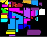
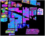
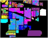
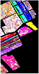
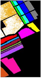
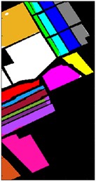
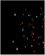
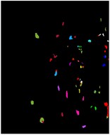
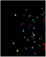
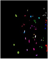
In Fig. 8 to Fig. 10, feature classification effects extracted by different schemes are given. Each color in the figure represents a feature category, and the classification of different features can be intuitively seen from the color figure.
Fig. 8Color diagram of Indian Pine classification
a) Color map
b) IMF1
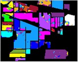
c) IMF2
d) IMF3
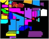
e) IMF4
f) Raw

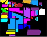
g) GA-IMF3

h) PSO-IMF3

i) BO-IMF3
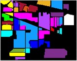
j) GWO-IMF3
Fig. 9Color diagram of Salians classification
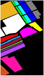
a) Color map
b) IMF1
c) IMF2

d) IMF3

e) IMF4
f) Raw

g) GA-IMF4

h) PSO-IMF4
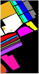
i) BO-IMF4
j) GWO-IMF4
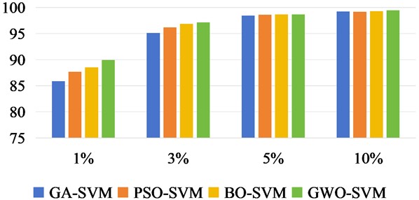
In Fig. 11 to Fig. 13, we increase the classification OA values of three datasets under different training samples. The results of each experiment were the mean after 10 times. According to the sample quantity of different data sets, 5 %, 8 %, 10 % and 15 % of the Indian Pine data set were taken as training samples respectively, and the rest were taken as test sets. For Salinas, 1 %, 2 %, 3 % and 5 % were taken as training sets. Take 1 %, 3 %, 5 % and 10 % of the KSC data set as the training set respectively.
Fig. 10Color diagram of KSC classification
a) Color map
b) IMF1

c) IMF2
d) IMF3
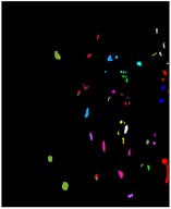
e) IMF4
f) Raw
g) GA-IMF4
h) PSO-IMF4

i) BO-IMF4
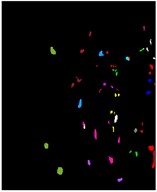
j) GWO-IMF4
Fig. 11Classification OA values of Indian Pine under different training sample datasets
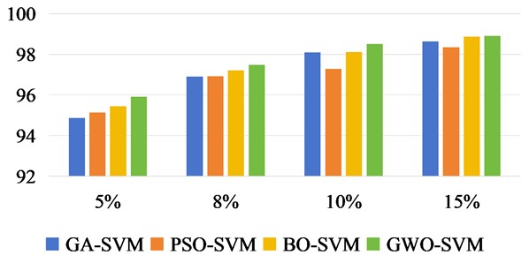
Fig. 12Classification OA values of Salinas under different training sample datasets
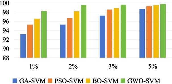
There was no overlap between the training and test samples in the three datasets. From the OA values of the classification effects of different training samples, we can intuitively see that the recognition accuracy of the three methods is constantly increasing with the increase of training samples. In Salinas data set, it can be seen that when the training sample is 2 %, the accuracy of OA classification has reached a better effect than that of GA-SVM, PSO-SVM and BO-SVM.
Fig. 13Classification OA values of KSC under different training sample datasets
5. Conclusions
This paper explores two main factors that affect the classification of HSIs. These two factors mainly include feature extraction and classifier network performance. Firstly, each band of the original HSIs data is processed by the feature extraction method of the spatial domain scheme. The optimal feature sample is found from the constructed new cube data set, and the best data sample is introduced into the optimized classifier network for new test. Through the recognition results of different ground object categories, it is found that the comprehensive consideration of the two factors of feature extraction and classifier recognition network optimization is more reasonable. It provides a feasible reference for further exploring the performance of HSIs classification.
References
-
M. P. Uddin, M. A. Mamun, and M. A. Hossain, “PCA-based feature reduction for hyperspectral remote sensing image classification,” IETE Technical Review, Vol. 38, No. 4, pp. 377–396, Jul. 2021, https://doi.org/10.1080/02564602.2020.1740615
-
D. M. Varade, A. K. Maurya, and O. Dikshit, “Development of spectral indexes in hyperspectral imagery for land cover assessment,” IETE Technical Review, Vol. 36, No. 5, pp. 475–483, Sep. 2019, https://doi.org/10.1080/02564602.2018.1503569
-
H. Wang, W. Li, X. Chen, and J. Niu, “Hyperspectral classification based on coupling multiscale super-pixels and spatial spectral features,” IEEE Geoscience and Remote Sensing Letters, Vol. 19, pp. 1–5, Jan. 2022, https://doi.org/10.1109/lgrs.2021.3086796
-
C. Zhao, C. Li, and S. Feng, “A spectral-spatial method based on fractional Fourier transform and collaborative representation for hyperspectral anomaly detection,” IEEE Geoscience and Remote Sensing Letters, Vol. 18, No. 7, pp. 1259–1263, Jul. 2021, https://doi.org/10.1109/lgrs.2020.2998576
-
H. Sun, X. Zheng, X. Lu, and S. Wu, “Spectral-spatial attention network for hyperspectral image classification,” IEEE Transactions on Geoscience and Remote Sensing, Vol. 58, No. 5, pp. 3232–3245, May 2020, https://doi.org/10.1109/tgrs.2019.2951160
-
B. Demir and S. Erturk, “Empirical mode decomposition of hyperspectral images for support vector machine classification,” IEEE Transactions on Geoscience and Remote Sensing, Vol. 48, No. 11, pp. 4071–4084, Nov. 2010, https://doi.org/10.1109/tgrs.2010.2070510
-
M. A. Shafaey et al., “Pixel-wise classification of hyperspectral images with 1D convolutional SVM networks,” IEEE Access, Vol. 10, pp. 133174–133185, Jan. 2022, https://doi.org/10.1109/access.2022.3231579
-
Y. Guo, X. Yin, X. Zhao, D. Yang, and Y. Bai, “Hyperspectral image classification with SVM and guided filter,” EURASIP Journal on Wireless Communications and Networking, Vol. 2019, No. 1, p. 56, Mar. 2019, https://doi.org/10.1186/s13638-019-1346-z
-
S. Zhang, H. Huang, Y. Huang, D. Cheng, and J. Huang, “A GA and SVM classification model for pine wilt disease detection using UAV-based hyperspectral imagery,” Applied Sciences, Vol. 12, No. 13, p. 6676, Jul. 2022, https://doi.org/10.3390/app12136676
-
A. Das and S. Patra, “A rough-GA based optimal feature selection in attribute profiles for classification of hyperspectral imagery,” Soft Computing, Vol. 24, No. 16, pp. 12569–12585, Jan. 2020, https://doi.org/10.1007/s00500-020-04697-y
-
Z. Xue, P. Du, and H. Su, “Harmonic analysis for hyperspectral image classification integrated with PSO optimized SVM,” IEEE Journal of Selected Topics in Applied Earth Observations and Remote Sensing, Vol. 7, No. 6, pp. 2131–2146, Jun. 2014, https://doi.org/10.1109/jstars.2014.2307091
-
C. Qi, Z. Zhou, Y. Sun, H. Song, L. Hu, and Q. Wang, “Feature selection and multiple kernel boosting framework based on PSO with mutation mechanism for hyperspectral classification,” Neurocomputing, Vol. 220, pp. 181–190, Jan. 2017, https://doi.org/10.1016/j.neucom.2016.05.103
-
X. Cao, J. Yao, X. Fu, H. Bi, and D. Hong, “An enhanced 3-D discrete wavelet transform for hyperspectral image classification,” IEEE Geoscience and Remote Sensing Letters, Vol. 18, No. 6, pp. 1104–1108, Jun. 2021, https://doi.org/10.1109/lgrs.2020.2990407
-
A. Ben Hamida, A. Benoit, P. Lambert, and C. Ben Amar, “3-D deep learning approach for remote sensing image classification,” IEEE Transactions on Geoscience and Remote Sensing, Vol. 56, No. 8, pp. 4420–4434, Aug. 2018, https://doi.org/10.1109/tgrs.2018.2818945
-
J. Xu, J. Zhao, and C. Liu, “An effective hyperspectral image classification approach based on discrete wavelet transform and dense CNN,” IEEE Geoscience and Remote Sensing Letters, Vol. 19, pp. 1–5, Jan. 2022, https://doi.org/10.1109/lgrs.2022.3181627
-
C. Yu, R. Han, M. Song, C. Liu, and C.-I. Chang, “A simplified 2D-3D CNN architecture for hyperspectral image classification based on spatial-spectral fusion,” IEEE Journal of Selected Topics in Applied Earth Observations and Remote Sensing, Vol. 13, pp. 2485–2501, Jan. 2020, https://doi.org/10.1109/jstars.2020.2983224
-
S. Mirjalili, S. M. Mirjalili, and A. Lewis, “Grey Wolf optimizer,” Advances in Engineering Software, Vol. 69, pp. 46–61, Mar. 2014, https://doi.org/10.1016/j.advengsoft.2013.12.007
About this article

This work is funded partly by Natural Science Foundation of Hunan Province of China under Grant No. 2021JJ60068, and partly by Hunan Province vocational college education and teaching reform research project under Grant No. ZJGB2022339, and partly by Hunan Province education science “14th Five-Year Plan” project under Grant No. XJK23CZY009.
The datasets generated during and/or analyzed during the current study are available from the corresponding author on reasonable request.
Jian Tang, major contributions are included the paper Conceptualization, Methodology and Writing. Dan Li, major contributions are included the paper Formal Analysis and Supervision. Lei Zhang, major contributions are included the paper Formal Analysis and Funding Acquisition. Xiangtong Nan, major contributions are included the paper Formal Analysis and Data Curation. Xin Li, major contributions include the paper Resources and Software. Dan Luo and Qianliang Xiao major contribution included the paper Funding Acquisition.
The authors declare that they have no conflict of interest.
