Abstract
Hyperspectral image (HSI) feature extraction is an important means to improve the classification of different ground features. According to the structural characteristics of hyperspectral data, the general feature extraction scheme can extract features from the point of view of spectral dimension, spatial and spatial spectrum. And the feature extraction time is also an index to measure the feature extraction method. Therefore, from the perspective of spatial dimension, this paper explores the relationship between HSI feature extraction time and training sample ratio. Three groups of HSIs sets were used for correlation test and analysis in the experiment. According to the characteristics of different data sets, the best selection scheme between spatial domain feature extraction method and training samples is given.
1. Introduction
Hyperspectral imaging (HSI) sensors can provide high-resolution spectral information from a wide range of the electromagnetic spectrum [1]. HSI technology provides better performance for classification and detection in remote sensing applications [2, 3]. The emergence of high spectral resolution airborne and satellite sensors has improved the ability to collect ground targets in different fields such as agriculture, geology, geography or national defense [4, 5]. HSI sensor has more advantages than multispectral sensor because its band spacing is narrow and it can collect hundreds of discrete frequency bands [6]. For most of these applications, feature extraction is a necessary processing step in order to obtain a more representative feature set and summarize the information in the HSI cube without losing any important information [7]. In order to avoid noise, curse of dimension, band information between redundant effects [8], one of the important research topics in the application of HSI in remote sensing is how to provide high classification accuracy. According to the classification unit, classification can be divided into object-oriented classification and pixel-based classification [9]. According to the form of classification, classification can be divided into supervised classification and unsupervised classification [10]. Under the condition of supervised classification, the effectiveness of pixel-based classification in support vector machine (SVM) HSI classification is verified [11]. Although spectral features are used as the main recognition features of HSI, spatial attributes are very useful to improve the accuracy of classification. Therefore, some feature extraction schemes based on spatial dimension are proposed. Literature [12] proposes to improve the classification accuracy based on SVM by using empirical mode decomposition (EMD) of HSI. The literature results show that EMD is especially suitable for nonlinear and non-stationary signals. EMD is used to decompose the bands of HSIs into several intrinsic mode functions (IMFs) and final residuals. By using EMD, the spatial adaptive decomposition of inherent features by EMD is effectively utilized, and the classification accuracy of HSIs is improved. Literature [13] proposes to use spectral gradient enhanced EMD to improve the classification accuracy of SVM for HSIs. In this paper, the classification accuracy can be significantly improved by using appropriate weights for IMF in the summation process. This method optimizes the total absolute spectral gradient by obtaining the weight of IMF, and uses the optimization strategy based on genetic algorithm to obtain the weight automatically. The experimental results show that this method can significantly improve the classification accuracy of HSIs. Literature [14] suggests that denoising should be combined with two-dimensional empirical mode decomposition (2D-EMD) of HSIs to improve the classification accuracy. Firstly, the band of HSI is decomposed into IMFs by 2D-EMD. Then, the first IMF of each frequency band is denoised, and then the features are reconstructed into the sum of low-order IMF for classification. A good classification effect is obtained in the SVM classifier. Reference [15] reports that the two-step method combining minimum noise component (MNF) and fast adaptive two-dimensional empirical mode decomposition (FABEMD) has been applied to improve the classification accuracy of airborne visible infrared imaging spectrometer HSIs of Indian Pine data set. After MNF dimensionality reduction, the HSI is decomposed into multiple two-dimensional intrinsic mode functions (BIMF) and residual images. Remove the first four BIMF, integrate the remaining BIMF to reconstruct the information image, and then classify it by SVM classifier. The classification results show that this method can effectively eliminate the influence of noise and achieve higher classification accuracy than traditional SVM. A new dimensionality reduction method for HSIs is proposed in reference [16]. It combines EMD with wavelet to produce the smallest feature set and obtain the best classification accuracy. The experimental results show that, compared with other direct dimensionality reduction methods based on frequency, the accuracy of feature classification obtained by this method is significantly improved. In reference [17], EMD and morphological wavelet transform (MWT) are used to obtain spectral spatial features. In the step of feature extraction, the sum of IMFs extracted by optimized EMD is taken as spectral features, while the spatial features are composed of low-frequency components of the first-order MWT. The experiment achieves good classification results. In order to deal with high-dimensional HSIs, a HSI classification method based on two-dimensional empirical wavelet transform (2D-EWT) feature extraction is proposed and compared with the image empirical mode decomposition (IEMD) method based on extracted features and original features [18]. This paper emphasizes that the number of features trained should be less than the number of features to be tested. Because the time of classification calculation is also the most important, only some fast and best classifiers are selected. In reference [19], the neural network model is used to forecast and analyze the data of river discharge. In literature [20], we used 2D-EMD spatial domain method to extract the spatial dimension feature information of HSIs, which greatly improved the classification performance of different ground objects. However, the time cost of spatial feature information extraction is neglected [21]. In this paper, SVM classifier is used, and the experimental results show that this method improves the performance of HSI classification in terms of classification evaluation index [22]. Other methods based on spatial domain are also widely studied and analyzed [23, 24].
The main contribution of this paper includes two aspects: (1) Comparing and analyzing the performance of two groups of spatial feature extraction methods in different data sets; (2) According to different HSIs characteristics, to explore the relationship between spatial domain feature extraction methods and training samples.
2. Methods
The realization of high classification effect of hyperspectral data mainly includes two factors. The first major factor is whether the feature sample contains the main feature information of the original cube. In general, when we classify, we first adopt feature extraction and preprocessing. The second major factor is the performance of the classifier. The performance of the classifier network also directly affects the classification results. In this paper, we explore two spatial domain feature extraction methods, 2D-EMD and 2D-EWT, and SVM classifier, which is commonly used in HSI classification.
2.1. Spatial domain feature extraction
According to the characteristics of data structure, HSI feature extraction can be carried out from the point of view of the combination of spectral domain, spatial domain and spatial spectral domain. After a lot of work, it is found that the angle feature extraction based on spatial domain has a greater improvement effect than the spectral dimension. Here we mainly analyze and introduce it from the perspective of spatial domain.
2.1.1. 2D-EMD
2D-EMD mainly deals with 2D signals, that is, 2D image data. 2D-EMD can decompose 2D images into several sub-band images from high frequency to low frequency. The high-frequency component contains the high-frequency detail information in the original image, while the low-frequency component contains the low-frequency information in the original image. For example, Eq. (1) indicates that a 2D image is decomposed into several intrinsic mode components and a remainder component:
where B represents a 2D image, and (i,j) represents the spatial location index of a 2D image. N denotes the number of sub-band images obtained by decomposition, and R denotes that the remainder sub-band images are obtained by decomposition.
2.1.2. 2D-EWT
The theoretical basis of 2D-EWT is established on the basis of traditional wavelet transform and EMD [25]. 2D-EWT can decompose 2D image into several coefficients, corresponding to approximate coefficients and detail coefficients respectively. The approximate coefficient corresponds to the low-frequency component of the original image, while the detail coefficient corresponds to the high-frequency detail component of the original image. Using the feature information contained in different coefficients, we can selectively select the coefficients to reconstruct different feature scale information in the original image. For example, Eqs. (2) and (3) indicate that a 2D image f is decomposed into approximate coefficients and detail coefficients. Specific technical details reference [25]:
There are many 2D empirical wavelet cluster schemes, among which we choose 2D empirical wavelet methods, 2D-Littlewood-Paley EWT (2D-LP-EWT) and 2D-Tensor-EWT (2D-T-EWT).
HSI is a cube structure, which can be regarded as superimposed by several 2D images. Each 2D image contains the characteristic information components of the corresponding band. Using the characteristics of 2D-EMD and 2D-EWT in processing 2D images, we will analyze them from the point of view of feature extraction in the spatial domain of HSIs. Each band of the HSI is decomposed into sub-band images from high frequency to low frequency, or the detail coefficient and approximation coefficient are obtained to reconstruct the feature information in the original image.
2.2. SVM classifier
Starting from some training samples, statistical learning theory tries to obtain some principles and rules that cannot be obtained by analyzing the samples. These rules are used to analyze objective objects and make more accurate predictions of unknown data. For given data, machine learning to find the relationship between input and output is the basis of our data analysis. There are many kinds of machine learning. Through machine learning, we can carry out regression analysis, classification analysis, cluster analysis and so on. SVM has a very good application effect in the analysis of small samples and nonlinear problems. In the application of hyperspectral image classification, SVM has been widely used and achieved good classification and recognition results [26-28].
However, SVM classifier has good performance and is highly dependent on related parameters. The two main parameters that have great influence on the effect of network classification are penalty factor parameters and kernel function parameters. When using kernel function for classification, how to select parameters is also an important direction of research, especially the parameters of penalty factor and kernel function directly affect the accuracy of prediction results. at present, there is no unified standard for the selection of parameters. in actual selection, many experiments are generally taken to find the optimal parameter value. The commonly used kernel functions are linear kernel function, polynomial kernel function, Gaussian radial basis kernel function, Sigmoid kernel function and so on. Generally, the selection of network penalty factor parameters and kernel function parameters can be optimized in the form of cross-validation, so as to obtain a better classification and recognition effect of SVM.
3. Introduction of experimental dataset and experimental scheme
3.1. Dataset
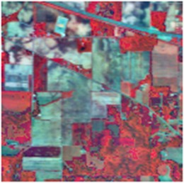
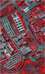
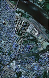
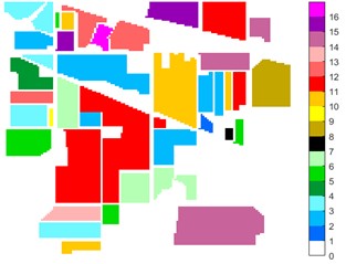
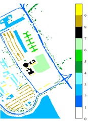
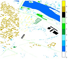
In this paper, three data sets are used to give the experimental results. Experimental data sources are available [29]. Indian Pine HSI is difficult to classify because the spectral features of different categories are highly similar and the pixels are highly mixed. These data consist of 145×145 pixels and 220 bands. By removing the bands covering water absorption zone and noise band, the number of bands is initially reduced to 200, containing a total of 16 feature categories. The second data set was obtained by the reflection Optical system Imaging Spectrometer sensor over the University of Pavia in northern Italy. The image consists of 103 spectral bands with a resolution of 610×340 pixels, a spectral coverage of 0.43-0.86 μ m and a spatial resolution of 1.3 m. Pavia University has a total of nine feature categories. The third data set is the remote sensing image of the Pavia Center. The number of spectral bands in the Pavia center is 102 and the resolution is 1096×715 pixel. There are a total of 9 feature categories. The number of samples for each category of the three sets of data sets and the corresponding category color map are shown in Fig. 1 and Table 1.
3.2. Experimental scheme
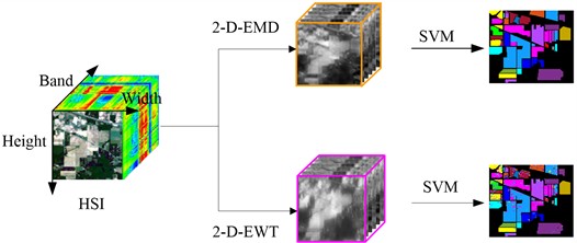
Fig. 2 shows the flow chart of spatial domain feature extraction and classification of HSIs. There are three main steps to this process. First, select the object we need to analyze and study, that is, select the data set for analysis. Here we selected Indian Pine, Pavia University and Pavia Centre, which are often used for experimental classification research. The second step is to decompose each band of hyperspectral data using spatial domain method. Supposed that the original hyperspectral dataset cube can be represented as RW×H×B, where W represents the width of the original cube structure, H represents the height of the original cube structure, and B represents the total number of bands of the original cube structure. The spatial domain decomposition method is used to operate on the 2D image of each band of HSI. Each 2D is equal in size, W and H in width and height. The decomposition of 2-D-EMD and 2-D-EWT is carried out from the first 2D band image successively until the decomposition of the last B-band image. The last step is to perform pixel-based SVM supervised classification on the new cube data set after spatial domain processing.
Table 1Groundtruth classes for the Indian Pine, Pavia University and Pavia Centre
Data | Indian Pine | Pavia University | Pavia Centre | |||
No. | Name | NoS | Name | NoS | Name | NoS |
1 | Alfalfa | 46 | Asphalt | 6631 | Water | 824 |
2 | Corn-notill | 1428 | Meadows | 18649 | Trees | 820 |
3 | Corn-mintill | 830 | Gravel | 2099 | Asphalt | 816 |
4 | Corn | 237 | Trees | 3064 | Self-Blocking Bricks | 808 |
5 | Grass-pasture | 483 | Painted metal sheets | 1345 | Bitumen | 808 |
6 | Grass-trees | 730 | Bare Soil | 5029 | Tiles | 1260 |
7 | Grass-pasture-mowed | 28 | Bitumen | 1330 | Shadows | 476 |
8 | Hay-windrowed | 478 | Self-Blocking Bricks | 3682 | Meadows | 824 |
9 | Oats | 20 | Shadows | 947 | Bare Soil | 820 |
10 | Soybean-notill | 972 | ||||
11 | Soybean-mintill | 2455 | ||||
12 | Soybean-clean | 593 | ||||
13 | Wheat | 205 | ||||
14 | Woods | 1265 | ||||
15 | Buildings-Grass-Trees-Drives | 386 | ||||
16 | Stone-Steel-Towers | 93 | ||||
Fig. 1Images of Indian Pine, Pavia university and Pavia Centre: a) Indian Pine RGB three-band map (R-G-B = 64-19-9); b) Indian Pine classification color map label; c) Pavia university RGB three-band map (R-G-B = 81-14-21); d) Pavia University classification color map label; e) Pavia Centre RGB three-band map (R-G-B = 11-31-42); f) Pavia Centre classification color map label
a)
c)
e)
b)
d)
f)
Fig. 2Flow chart of spatial feature extraction and classification of HSI
3.3. Metric
The Overall Accuracy (OA) classification accuracy refers to the percentage of the number of correctly classified pixels in the entire image. Through this index, the quality of the classification results can be intuitively seen. The definition is as follows:
The average accuracy (AA) refers to the average of classification accuracy of various categories, which can measure the influence of categories on classification accuracy, and its definition is as follows:
The Kappa coefficient fully considers the impact of uncertainty on classification results, is used to test the degree of consistency, and can objectively measure the overall result of classification. Its definition is as follows:
where, N represents the total sample number, ci+ represents the real pixel number of class i, and c+i represents the pixel number classified into class i during prediction. The Kappa coefficient is a ratio that represents the reduction in errors between a classification and a completely random classification.
4. Experimental simulation and discussion
4.1. Classified test
After feature extraction in spatial domain, HSIs are supervised and classified by SVM. The extracted feature samples are divided into training set and test set, and the corresponding label operations are carried out on the samples. Here, we use pixels as the basic unit for HSI hard classification. The widely used OA, AA and Kappa coefficients are used in the test and evaluation criteria. Each experiment is the result of 10 times average. SVM network training uses cross-validation to optimize the parameters of penalty factor and kernel function. Here, the widely used radial basis kernel function is used as the kernel function.
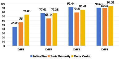
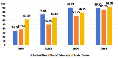
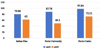
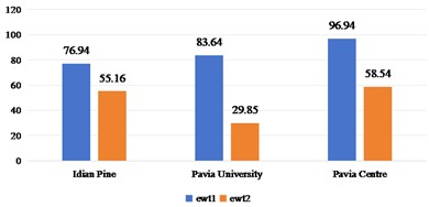
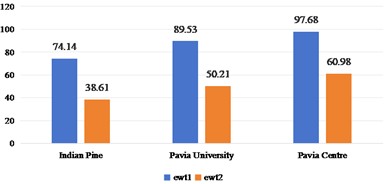
2D-EMD and 2D-EWT can decompose each band of a HSI into several intrinsic mode components (or approximate coefficients and detail coefficients). Therefore, we first discuss the sub-band images obtained by 2D-EMD and 2D-EWT decomposition for recognition and analysis. Considering that there are many kinds of 2D-EWT families, we discuss the effects of 2D-LP-EWT and 2D-T-EWT. The 2D-EWD decomposes three sets of data sets into four intrinsic pattern components. In Fig. 3, we show the recognition effect of four intrinsic pattern components. From the recognition results, the OA and Kappa values of the third intrinsic pattern component are the best in the Indian Pine data set. The fourth intrinsic pattern component of Pavia University and Pavia Centre has the best classification effect of OA and Kappa. Generally speaking, the effect of low-order intrinsic mode components is better, indicating that the features in low-order sub-band images are more helpful to distinguish different features. In Figs. 4 and 5, the effect of feature recognition and classification of the first sub-band and the second sub-band image obtained by 2D-LP-EWT and 2D-T-EWT decomposition is shown. From the point of view of the recognition effect, the recognition effect of the first approximate coefficient is better in the three sets of data sets. The approximate coefficient contains the feature information which is more beneficial to classification.
Based on the analysis of the feature information of different sub-band images obtained by 2D-EMD and 2D-EWT decomposition, we come to the conclusion that the feature information contained in low-frequency sub-band images and approximate coefficient sub-bands is more beneficial to improve the classification performance. We will analyze the classification performance of optimal low-frequency sub-band images and approximate coefficient sub-bands on different training samples.
Fig. 3Spatial domain feature extraction and classification results of 2D-EMD on three sets of data sets
a)OA
b) Kappa
Fig. 4Spatial domain feature extraction and classification results of 2D-LP-EWT on three sets of data sets
a)OA
b) Kappa
Fig. 5Spatial domain feature extraction and classification results of 2D-T-EWT on three sets of data sets
a)OA
b) Kappa
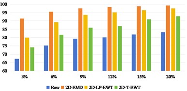
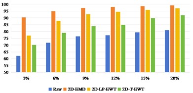
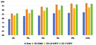
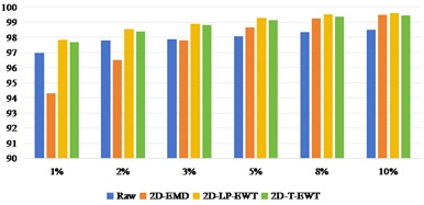
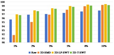
Fig. 6-8 shows the best sub-band image classification results of three sets of data sets in different methods, as well as the recognition OA and Kappa values under different training samples. Fig. 6 shows the result of Indian Pine recognition, from which we can see that the direct classification effect of the original data set is very poor. After the feature extraction in spatial domain, the recognition effect is improved. In addition, the recognition effect gap between different spatial domain methods is also obvious. The recognition effect of 2D-EMD is the best, followed by 2D-LP-EWT. When the training sample interval is 3 %-12 %, the difference between 2D-EMD and 2D-LP-EWT recognition effect is obvious. With the continuous increase of training samples, when the training samples reach 20 %, the gap between the two is getting smaller and smaller.
With the increase of training samples, the OA and Kappa values of recognition results also increase. By adding training samples, useful classification feature information can be increased to a certain extent, so as to improve the robustness of network training and further improve the effect of recognition and classification.
Fig. 6OA and Kappa values of recognition results of Indian Pine data sets under different training samples
a)OA
b) Kappa
Fig. 7OA and Kappa values of recognition results of Pavia University data sets under different training samples
a)OA
b) Kappa
Fig. 8OA and Kappa values of recognition results of Pavia Centre data sets under different training samples
a)OA
b) Kappa
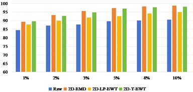
Fig. 7 shows the result of Pavia U recognition, from which we can see that the direct classification effect of the original data set is better than that of India Pine. After three kinds of spatial domain feature extraction, the recognition effect has been obviously improved. The recognition effect of 2D-EMD is similar to that of 2D-T-EWT, while the recognition effect of 2D-LP-EWT is relatively poor.
Fig. 8 shows the results of Pavia Centre recognition, from which we can see that the effect of direct classification is better than that of Indian Pine and Pavia U. It shows that it is less difficult to extract features from Pavia Centre data sets. When the training sample interval is between 1 % and 3 %, the recognition effect of 2D-EMD method is not as good as that of Raw direct classification. After the training sample interval is 5 %, the effect advantage of 2D-EMD feature extraction can be highlighted, indicating that after increasing the training samples, the feature information that can be used to improve the classification is added. On the other hand, 2D-LP-EWT and 2D-T-EWT are improved in all datasets. The classification effect between the two is similar.
4.2. Feature extraction time
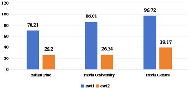
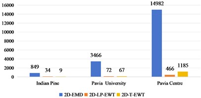
Under the condition of considering different spatial domain feature extraction methods and different training sample classification results, we further compare the time cost of different spatial domain feature extraction methods. Fig. 9 shows the time cost of the three sets of data. Generally speaking, the time cost of Indian Pine is shorter and that of Pavia Centre is longer, which is mainly determined by the band size and the total number of bands of the data set. Compared with the 2D-EMD method, the time cost of 2D-EWT is shorter, which can greatly save the time of feature extraction.
Fig. 9Time cost of feature extraction methods in different spatial domains
4.3. Discussion
According to the characteristics of different hyperspectral data sets, choosing the appropriate spatial domain feature extraction method not only needs to consider to improve the actual classification effect, but also needs to consider the time cost of feature extraction. For the Indian Pine dataset, we conclude that 2D-EMD is a better choice when the training sample interval is 1 % to 20 %. When the training sample is more than 20 %, it is the best choice to use 2D-LP-EWT method to extract features to the first approximate coefficient for classification. It is the best choice to use 2D-T-EWT for feature extraction and classification for Pavia U data sets. Using 2D-LP-EWT for feature extraction and classification is the best choice for Pavia Centre data sets.
4.4. Classified color map
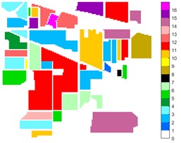
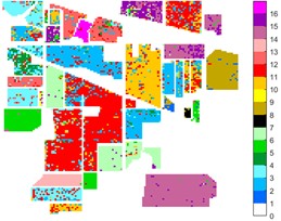
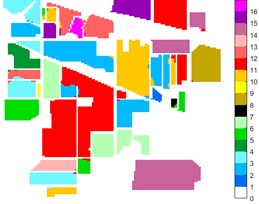
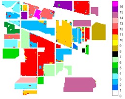
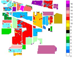
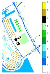
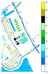
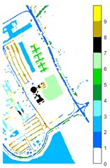
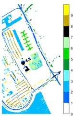
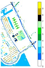
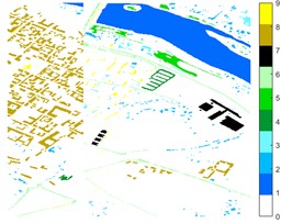
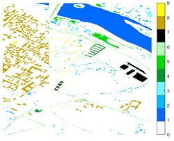
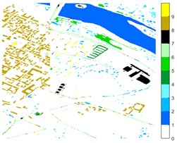
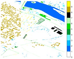
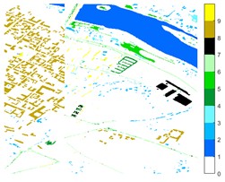
Figs. 10-12 shows the classification of three sets of data sets under different feature extraction. Fig. 10 shows the comparison results of the classified color images of Indian Pine when the training samples are 10 %. Fig. 10 sub-image (a) is the reference image we compared. The closer the other sub-images are to the sub-image (a), the better the recognition effect is, and the better the feature extraction method is. It can be seen from the subgraph that the recognition effect of the subgraph (c) is closer to that of the subgraph (a). The OA, AA and Kappa values for different features are given in Table 2. The results of each experiment are the average results after 10 times. Similarly, Figs. 11 and 12 show the recognition color diagrams of Pavia U and Pavia Centre, respectively. Table 3 and Table 4 show the classification OA, AA and Kappa values of different features, respectively. In Table 3 and Table 4, 2D-EWT and 2D-EMD spatial domain feature extraction methods show great differences in the classification results of different ground objects.
Fig. 10Indian Pine different feature classification color maps under different feature extraction methods
a) Colour map
b) Raw
c) 2D-EMD
d) 2D-LP-EWT
e) 2D-T-EWT
Table 2Different feature classification OA, AA and Kappa values of Indian Pine under different spatial domain feature extraction methods
– | Raw | 2D-EMD | 2D-LP-EWT | 2D-T-EWT |
C1 | 70.24±12.85 | 87.80±15.5 | 92.68±4.08 | 76.10±22.69 |
C2 | 76.34±3.76 | 97.21±0.82 | 89.99±2.43 | 83.75±3.44 |
C3 | 62.36±6.56 | 98.55±0.48 | 91.16±1.82 | 77.46±4.23 |
C4 | 47.32±12.36 | 96.72±2.18 | 89.67±2.08 | 76.06±3.99 |
C5 | 89.84±2.46 | 96.41±2.44 | 94.21±1.73 | 93.89±1.99 |
C6 | 95.04±1.28 | 99.30±0.67 | 98.60±1.26 | 99.00±1.13 |
C7 | 73.6±7.84 | 88.00±16.0 | 82.40±64.50 | 70.40±7.84 |
C8 | 95.44±1.13 | 99.53±0.49 | 99.21±1.17 | 99.35±0.61 |
C9 | 23.33±5.44 | 87.78±7.37 | 84.44±12.37 | 73.33±15.48 |
C10 | 67.66±2.70 | 95.63±1.74 | 88.07±5.77 | 76.34±5.02 |
C11 | 80.79±3.10 | 98.61±0.38 | 94.08±1.03 | 86.50±2.64 |
C12 | 68.61±4.54 | 94.61±2.04 | 87.57±3.95 | 79.83±2.03 |
C13 | 97.28±0.34 | 96.30±3.72 | 99.35±0.80 | 98.80±0.80 |
C14 | 95.59±1.73 | 99.40±0.42 | 99.65±0.36 | 96.27±1.54 |
C15 | 50.84±9.18 | 97.98±1.20 | 98.39±1.19 | 79.37±4.19 |
C16 | 93.33±2.67 | 92.14±5.71 | 97.86±2.18 | 96.19±4.42 |
AA | 74.23±2.12 | 95.37±1.86 | 92.96±1.45 | 85.17±2.16 |
OA | 74.35±0.76 | 97.71±0.37 | 93.72±1.05 | 86.79±1.27 |
Kappa×100 | 75.21±0.91 | 97.39±0.42 | 92.84±1.21 | 84.91±1.46 |
In Table 3, C6 and C9 respectively represent the classification effect of the 6th and 9th type of feature, indicating that 2D-EMD is more effective in extracting spatial dimensional feature information of the 6th type of feature. However, for the feature extraction effect of the 9th ground object, 2D-EWT method will be more advantageous. It shows that different spatial dimension feature extraction methods show different differences in solving the problem of the same object with different spectrum and the same spectrum foreign object. At the same time, in Pavia Centre data, the 2D-EMD method also has a large room for improvement in the extraction effect of the 9th type of ground feature.
Fig. 11Pavia U color maps of different ground features under different feature extraction methods
a) Colour map
b) Raw
c) 2D-EMD
d) 2D-LP-EWT
e) 2D-T-EWT
Fig. 12Pavia Centre different feature classification color maps under different feature extraction methods
a) Colour map
b) Raw
c) 2D-EMD
d) 2D-LP-EWT
e) 2D-T-EWT
Table 3The OA, AA and Kappa values of different feature classification of Pavia U under different spatial domain feature extraction methods
– | Raw | 2D-EMD | 2D-LP-EWT | 2D-T-EWT |
C1 | 84.02±2.45 | 81.00±2.81 | 84.79±1.07 | 89.92±2.13 |
C2 | 94.81±1.28 | 99.37±0.19 | 97.85±0.95 | 97.63±0.87 |
C3 | 60.83±4.87 | 86.39±2.88 | 58.29±8.75 | 72.40±5.19 |
C4 | 86.20±2.51 | 53.04±5.37 | 94.07±2.09 | 85.05±2.26 |
C5 | 99.16±0.36 | 86.58±8.93 | 99.35±0.33 | 99.10±0.61 |
C6 | 62.55±5.99 | 97.69±1.84 | 72.28±2.93 | 82.90±2.15 |
C7 | 66.53±8.84 | 93.33±5.00 | 65.44±5.70 | 56.78±9.85 |
C8 | 81.36±4.86 | 84.07±5.33 | 75.74±3.23 | 79.83±3.59 |
C9 | 92.77±1.88 | 36.52±6.18 | 95.76±1.14 | 86.95±3.58 |
AA | 80.91±0.94 | 79.77±1.49 | 82.62±1.60 | 83.40±1.05 |
OA | 85.11±0.34 | 89.07±0.48 | 87.70±0.48 | 89.57±0.49 |
Kappa×100 | 80.01±0.45 | 85.44±0.65 | 83.49±0.69 | 86.07±0.63 |
Table 4Different feature classification OA, AA and Kappa values of Pavia Centre under different spatial domain feature extraction methods
– | Raw | 2D-EMD | 2D-LP-EWT | 2D-T-EWT |
C1 | 99.95±0.02 | 99.91±0.11 | 99.94±0.04 | 99.93±0.05 |
C2 | 93.65±0.58 | 84.52±1.92 | 93.78±0.46 | 92.48±1.13 |
C3 | 80.63±2.54 | 76.64±6.72 | 86.66±2.87 | 84.96±4.08 |
C4 | 72.44±3.75 | 89.32±1.68 | 89.98±3.88 | 85.64±6.05 |
C5 | 92.59±1.47 | 89.84±0.77 | 94.88±2.09 | 97.70±1.07 |
C6 | 89.50±4.53 | 77.11±3.56 | 92.09±1.95 | 87.39±2.61 |
C7 | 89.75±2.02 | 97.28±1.97 | 89.33±2.23 | 90.65±1.13 |
C8 | 99.14±0.21 | 95.96±1.05 | 99.69±0.07 | 99.75±0.03 |
C9 | 93.66±0.93 | 44.58±3.51 | 96.49±0.63 | 94.56±1.16 |
AA | 90.15±0.89 | 83.91±0.91 | 93.65±0.97 | 92.56±0.33 |
OA | 96.89±0.31 | 94.23±0.38 | 97.79±0.32 | 97.48±0.06 |
Kappa×100 | 95.60±0.44 | 91.84±0.53 | 96.87±0.45 | 96.43±0.09 |
5. Conclusions
Combined with the widely used spatial domain feature extraction methods of HSIs, this paper explores the relationship between 2D-EMD, 2D-LP-EWT and 2D-T-EWT spatial domain feature extraction and training samples. According to the characteristics of different data sets of HSIs, the characteristics of different data sets under different spatial domain feature extraction methods are given, including the classification performance comparison of different sub-band images obtained by decomposition. It includes the recognition of classification effect under different training samples, and the comprehensive measurement and analysis of the feature extraction time of decomposition. It provides a general analysis idea for feature extraction in spatial domain of different HSIs. The quality of feature extraction has a direct correlation with the classification performance of different ground objects. However, while we consider analytical feature extraction, time evaluation is also a crucial metric. The next task is how to select the corresponding spatial feature extraction methods according to the characteristics of different remote sensing images, and how to achieve a relative balance between time performance and feature extraction effect performance.
References
-
B. Lu, P. Dao, J. Liu, Y. He, and J. Shang, “Recent advances of hyperspectral imaging technology and applications in agriculture,” Remote Sensing, Vol. 12, No. 16, p. 2659, Aug. 2020, https://doi.org/10.3390/rs12162659
-
D. Hong et al., “SpectralFormer: rethinking hyperspectral image classification with transformers,” IEEE Transactions on Geoscience and Remote Sensing, Vol. 60, pp. 1–15, Jan. 2022, https://doi.org/10.1109/tgrs.2021.3130716
-
H. Chen, F. Miao, Y. Chen, Y. Xiong, and T. Chen, “A hyperspectral image classification method using multifeature vectors and optimized KELM,” IEEE Journal of Selected Topics in Applied Earth Observations and Remote Sensing, Vol. 14, pp. 2781–2795, Jan. 2021, https://doi.org/10.1109/jstars.2021.3059451
-
S. Hou, H. Shi, X. Cao, X. Zhang, and L. Jiao, “Hyperspectral imagery classification based on contrastive learning,” IEEE Transactions on Geoscience and Remote Sensing, Vol. 60, pp. 1–13, Jan. 2022, https://doi.org/10.1109/tgrs.2021.3139099
-
D. Hong, L. Gao, J. Yao, B. Zhang, A. Plaza, and J. Chanussot, “Graph convolutional networks for hyperspectral image classification,” IEEE Transactions on Geoscience and Remote Sensing, Vol. 59, No. 7, pp. 5966–5978, Jul. 2021, https://doi.org/10.1109/tgrs.2020.3015157
-
Q. Shi, X. Tang, T. Yang, R. Liu, and L. Zhang, “Hyperspectral image denoising using a 3-D attention denoising network,” IEEE Transactions on Geoscience and Remote Sensing, Vol. 59, No. 12, pp. 10348–10363, Dec. 2021, https://doi.org/10.1109/tgrs.2020.3045273
-
F. Luo, Z. Zou, J. Liu, and Z. Lin, “Dimensionality reduction and classification of hyperspectral image via multistructure unified discriminative embedding,” IEEE Transactions on Geoscience and Remote Sensing, Vol. 60, pp. 1–16, Jan. 2022, https://doi.org/10.1109/tgrs.2021.3128764
-
Zhang C. et al., “Noise reduction in the spectral domain of hyperspectral images using denoising autoencoder methods,” Chemometrics and Intelligent Laboratory Systems, Vol. 203, p. 104063, 2020, https://doi.org/10.1016/j.chemolab.2020.10406
-
O. Okwuashi and C. E. Ndehedehe, “Deep support vector machine for hyperspectral image classification,” Pattern Recognition, Vol. 103, p. 107298, Jul. 2020, https://doi.org/10.1016/j.patcog.2020.107298
-
S. Wan, M.-L. Yeh, and H.-L. Ma, “An innovative intelligent system with integrated CNN and SVM: considering various crops through hyperspectral image data,” ISPRS International Journal of Geo-Information, Vol. 10, No. 4, p. 242, Apr. 2021, https://doi.org/10.3390/ijgi10040242
-
X. Cao, D. Wang, X. Wang, J. Zhao, and L. Jiao, “Hyperspectral imagery classification with cascaded support vector machines and multi-scale superpixel segmentation,” International Journal of Remote Sensing, Vol. 41, No. 12, pp. 4530–4550, Jun. 2020, https://doi.org/10.1080/01431161.2020.1723172
-
B. Demir and S. Erturk, “Empirical mode decomposition of hyperspectral images for support vector machine classification,” IEEE Transactions on Geoscience and Remote Sensing, Vol. 48, No. 11, pp. 4071–4084, Nov. 2010, https://doi.org/10.1109/tgrs.2010.2070510
-
A. Erturk, M. K. Gullu, and S. Erturk, “Hyperspectral image classification using empirical mode decomposition with spectral gradient enhancement,” IEEE Transactions on Geoscience and Remote Sensing, Vol. 51, No. 5, pp. 2787–2798, May 2013, https://doi.org/10.1109/tgrs.2012.2217501
-
B. Demir, S. Erturk, and M. K. Gullu, “Hyperspectral image classification using denoising of intrinsic mode functions,” IEEE Geoscience and Remote Sensing Letters, Vol. 8, No. 2, pp. 220–224, Mar. 2011, https://doi.org/10.1109/lgrs.2010.2058996
-
M.-D. Yang, K.-S. Huang, Y. F. Yang, L.-Y. Lu, Z.-Y. Feng, and H. P. Tsai, “Hyperspectral image classification using fast and adaptive bidimensional empirical mode decomposition with minimum noise fraction,” IEEE Geoscience and Remote Sensing Letters, Vol. 13, No. 12, pp. 1950–1954, Dec. 2016, https://doi.org/10.1109/lgrs.2016.2618930
-
E. T. Gormus, N. Canagarajah, and A. Achim, “Dimensionality reduction of hyperspectral images using empirical mode decompositions and wavelets,” IEEE Journal of Selected Topics in Applied Earth Observations and Remote Sensing, Vol. 5, No. 6, pp. 1821–1830, Dec. 2012, https://doi.org/10.1109/jstars.2012.2203587
-
Zhi He, Qiang Wang, Yi Shen, and Mingjian Sun, “Kernel sparse multitask learning for hyperspectral image classification with empirical mode decomposition and morphological wavelet-based features,” IEEE Transactions on Geoscience and Remote Sensing, Vol. 52, No. 8, pp. 5150–5163, Aug. 2014, https://doi.org/10.1109/tgrs.2013.2287022
-
T. V. N. Prabhakar and P. Geetha, “Two-dimensional empirical wavelet transform based supervised hyperspectral image classification,” ISPRS Journal of Photogrammetry and Remote Sensing, Vol. 133, pp. 37–45, Nov. 2017, https://doi.org/10.1016/j.isprsjprs.2017.09.003
-
C. Pany, U. K. Tripathy, and L. Misra, “Application of artificial neural network and autoregressive model in stream flow forecasting,” Journal-Indian Waterworks Association, Vol. 33, No. 1, pp. 61–68, 2001.
-
J. Tang et al., “Feature extraction of hyperspectral images based on SVM optimization of 2D-EMD and GWO,” Journal of Measurements in Engineering, Vol. 12, No. 4, Aug. 2024, https://doi.org/10.21595/jme.2024.23844
-
W. Xie, Y. Gu, and T. Liu, “Hyperspectral intrinsic image decomposition based on physical prior-driven unsupervised learning,” IEEE Transactions on Geoscience and Remote Sensing, Vol. 61, pp. 1–14, Jan. 2023, https://doi.org/10.1109/tgrs.2023.3281490
-
J. Zabalza et al., “Novel two-dimensional singular spectrum analysis for effective feature extraction and data classification in hyperspectral imaging,” IEEE Transactions on Geoscience and Remote Sensing, Vol. 53, No. 8, pp. 4418–4433, Aug. 2015, https://doi.org/10.1109/tgrs.2015.2398468
-
G. Sun et al., “SpaSSA: superpixelwise adaptive SSA for unsupervised spatial-spectral feature extraction in hyperspectral image,” IEEE Transactions on Cybernetics, Vol. 52, No. 7, pp. 6158–6169, Jul. 2022, https://doi.org/10.1109/tcyb.2021.3104100
-
H. Fu, G. Sun, J. Ren, A. Zhang, and X. Jia, “Fusion of PCA and segmented-PCA domain multiscale 2-D-SSA for effective spectral-spatial feature extraction and data classification in hyperspectral imagery,” IEEE Transactions on Geoscience and Remote Sensing, Vol. 60, pp. 1–14, Jan. 2022, https://doi.org/10.1109/tgrs.2020.3034656
-
J. Gilles, G. Tran, and S. Osher, “2D empirical transforms. wavelets, ridgelets, and curvelets revisited,” SIAM Journal on Imaging Sciences, Vol. 7, No. 1, pp. 157–186, Jan. 2014, https://doi.org/10.1137/130923774
-
G. Liu, L. Wang, D. Liu, L. Fei, and J. Yang, “Hyperspectral image classification based on non-parallel support vector machine,” Remote Sensing, Vol. 14, No. 10, p. 2447, May 2022, https://doi.org/10.3390/rs14102447
-
Y. Guo, X. Yin, X. Zhao, D. Yang, and Y. Bai, “Hyperspectral image classification with SVM and guided filter,” EURASIP Journal on Wireless Communications and Networking, Vol. 2019, No. 1, pp. 1–9, Mar. 2019, https://doi.org/10.1186/s13638-019-1346-z
-
M. A. Shafaey et al., “Pixel-wise classification of hyperspectral images with 1D convolutional SVM networks,” IEEE Access, Vol. 10, pp. 133174–133185, Jan. 2022, https://doi.org/10.1109/access.2022.3231579
-
Hyperspectral Remote Sensing Scenes,” https://www.ehu.eus/ccwintco/index.php?title=hyperspectral_remote_sensing_scenes
About this article
This research was funded by Natural Science Foundation of Hunan Province of China, grant number 2024JJ8019 and 2021JJ60068.
The datasets generated during and/or analyzed during the current study are available from the corresponding author on reasonable request.
Jian Tang: methodology. Dan Li: conceptualization. Hongbing Liu: formal analysis. Xiaochun Liu: validation. Dan Luo: funding acquisition. Hong Zhou: visualization. Hongyan Cui: software. Qianliang Xiao: funding acquisition.
The authors declare that they have no conflict of interest.

