Abstract
In response to the significant challenges posed by strong non-stationarity and the vulnerability to intense background noise in rolling bearing signals, as well as the inherent limitations of conventional convolutional neural networks (CNN) when processing one-dimensional (1D) signals without fully leveraging the inter-data relationships, this study introduces an innovative diagnostic approach for rolling bearings. The method employs the Time-Reassigned Multi-Synchro Squeezing Transform (TMSST) to preprocess 1D vibration signals. By harnessing the temporal correlations across various intervals, TMSST generates a set of time-frequency feature maps that are subsequently fed into a CNN to adaptively extract and classify the fault characteristics of rolling bearings. To substantiate the efficacy of the proposed model, the Case Western Reserve University's bearing dataset serves as the benchmark for the fault diagnosis analysis. Moreover, the study incorporates several alternative data processing techniques for comparative evaluation of the classification accuracy. The findings reveal that the proposed model, when juxtaposed with other image encoding methods, consistently delivers superior diagnostic performance across a spectrum of load conditions and noise environments. It achieves an impressive global accuracy of 95.67 %, thereby facilitating robust end-to-end fault pattern recognition in rolling bearings.
Highlights
- This paper presents a groundbreaking TMSST-CNN model that achieves a remarkable diagnostic accuracy of 95.67% for rolling bearing faults.
- The research demonstrates significant performance improvements in the model's diagnostic precision through the application of reinforcement learning.
- Comparative analysis shows that the TMSST image encoding technique surpasses other methods in fault diagnosis.
1. Introduction
Rolling bearings, integral to the rotating machinery, exert a pivotal influence on the operational stability and longevity of the mechanism under diverse loading and positional scenarios. The real-time surveillance of the vibration signals emanating from the machinery is of paramount importance for its stable function, offering maintenance personnel an all-encompassing assessment of the equipment's operational status [1]. However, the conventional fault diagnosis techniques, which are predominantly dependent on the manual analysis by experts, have proven to be insufficient in tackling the challenges of voluminous, heterogeneous, and rapid data streams characteristic of the modern machinery industry. Specifically, in the context of vast datasets from mechanical equipment under fluctuating operational conditions, the traditional methods often encounter limitations in their monitoring capabilities and generalization performance, particularly when faced with intricate and mutable fault information [2]. Consequently, the integration of mechanical equipment data with intelligent algorithms to forge intelligent fault diagnosis technologies has emerged as an essential strategy to surmount these challenges [3].
The conventional intelligent fault diagnosis process is typically structured around three fundamental stages: Initially, signal acquisition is executed through sensors and related devices to gather foundational data on the machinery's operational status. Subsequently, signal processing methodologies are applied to distill features from the acquired signals, thereby uncovering the characteristic information indicative of equipment faults. Ultimately, leveraging the extracted feature data, machine learning (ML) or deep learning (DL) algorithms are engaged for fault identification, ascertaining the nature and severity of the equipment's faults [4]. By amalgamating intelligent algorithms with mechanical equipment data, intelligent fault diagnosis methods not only enhance the precision and efficiency of fault diagnosis but also promote predictive maintenance, thereby providing a solid foundation for the secure and stable operation of mechanical equipment [5].
The 1D vibration signals of rolling bearings encapsulate a wealth of information regarding their operational status, characterized by their inherent nonlinearity and non-stationarity. Consequently, the extraction of fault features stands as an indispensable step in the realm of fault diagnosis [6]. Time-frequency analysis emerges as a robust signal processing technique that concurrently examines both temporal and spectral aspects of a signal. The spectrum of common time-frequency analysis methods encompasses Empirical Mode Decomposition (EMD) [7], Short-Time Fourier Transform (STFT) [8], and Wavelet Transform (WT) [9]. EMD offers the capability to adaptively decompose signals into a series of Intrinsic Mode Functions (IMFs) that represent different scale-specific components. However, the process may encounter the problem of mode mixing, leading to inaccurate decomposition and affecting subsequent analysis and judgment. STFT, while adept at conducting time-frequency analysis, is constrained by its fixed time resolution, which may not adequately capture the abrupt transitions present in vibration signals. This characteristic results in STFT losing some feature quantities, leading to misjudgment of bearing fault signals. Conversely, WT is distinguished by its variable time window that contracts with increasing signal frequency and expands otherwise, thereby extending the capabilities of STFT and mitigating its inherent limitations, which has led to its broad adoption in various applications. However, when processing signals with complex spectra, it may not provide accurate analysis results, which can lead to misjudgment or missed judgment when analyzing bearing fault characteristics.
Yan et al. have provided a comprehensive review of the applications of Continuous Wavelet Transform (CWT), Discrete Wavelet Transform (DWT), Wavelet Packet Transform (WPT), and Second-Generation Wavelet Transform (SGWT) within the domain of fault diagnosis [10]. TMSST is a signal processing technique particularly suited for processing nonlinear and non-stationary signals. It is an improvement based on the traditional SST. Through time reassignment technology, TMSST further processes signals to improve the accuracy and resolution of time-frequency analysis. Time reassignment can reduce cross-terms in time-frequency representation, thereby more clearly revealing the intrinsic structure of the signal. By adjusting the time axis of the signal, the time-frequency representation of the signal becomes more focused, making it easier to identify and extract fault characteristics. In parallel, fault recognition is equally pivotal in the diagnostic process, as mere feature extraction is insufficient for handling the demands of voluminous data processing. Traditional fault recognition tools encompass Bayesian classifiers [11], Artificial Neural Networks (ANNs) [12, 13], and Support Vector Machines (SVMs). Both Bayesian classifiers and ANNs are adept at discerning fault types, provided that a substantial number of training samples are at their disposal. However, procuring an ample dataset of fault samples in practical scenarios can be quite challenging. SVMs, endowed with robust generalization capabilities, commendable versatility, and high classification precision, are capable of achieving effective classification even with a modest number of samples, which has propelled their widespread application in the research of mechanical fault diagnosis [14-17]. Nonetheless, SVMs may underperform with redundant data due to their inherent limitations in learning deep features, attributed to their shallow architecture [18].
The unprecedented success of CNN in the domain of image classification has spurred significant interest in transforming sensor-collected signals into image-based representations through specialized encoding techniques, a topic that is currently at the forefront of research [19]. Tao et al. have pioneered a method that amalgamates Short-Time Fourier Transform (STFT) with Classification Generative Adversarial Networks (cGAN) to transmute 1D signals into two-dimensional (2D) time-frequency images, thereby achieving commendable diagnostic accuracy [20]. Yuan et al. have harnessed the Hilbert-Huang Transform (HHT) to translate the temporal sequences of vibration signals into time-frequency images, subsequently employing a CNN to discern fault-sensitive features within the time-frequency spectrum from these images for fault classification [21]. Zheng et al. introduced a novel Multi-Synchronous Compression S-Transform, integrating the S-Transform within a multi-synchronous compression framework, and substantiated the efficacy of this approach through both simulated and field signals [22]. In addition, Zhou et al. have presented a rolling bearing diagnosis methodology predicated on the Wigner-Ville Distribution (WVD) [23]. These methodologies underscore the potential of transmuting vibration signals into image representations for fault diagnosis via CNNs. By capitalizing on the prodigious feature extraction process of CNNs, it becomes feasible to distill meaningful insights from time-frequency images and classify various fault types with precision. This investigative trajectory is replete with promise for augmenting the fidelity and expedience of mechanical fault diagnosis systems.
This paper introduces an innovative TMSST-CNN model. which offers significant improvements in signal transformation and fault recognition. TMSST is used to convert raw data into feature-rich images without relying on preset parameters, effectively extracting useful information from these complex signals. Subsequently, these feature maps can be combined with CNN to further enhance the accuracy of fault diagnosis by leveraging CNN's powerful feature extraction capabilities after transforming the signals into images. The proposed methodology’s efficacy is corroborated using rolling bearing data procured from the Case Western Reserve University Bearing Data Center and Fault Diagnosis Prototype Rig. Moreover, the model’s generalization capability is rigorously tested across a variety of load conditions and noisy environments. The findings indicate that the TMSST-CNN model surpasses alternative 2D image encoding techniques in the realm of rolling bearing fault diagnosis, attaining an accuracy of 95.67 %.
2. Time-reassigned multi-synchro squeezing transform
2.1. Time-reassigned synchro squeezing transform
In this section, we first briefly introduce the theoretical basis of the TSST [24]. A single-component signal with varying frequency can be described in Eq. (1):
where, and represent the amplitude and phase of the signal in the frequency domain, while denotes the group delay (GD). When a signal is represented in the time-frequency domain, the Ideal Time-frequency Representation (ITFR) can be expressed as Eq. (2):
where, represents the Dirac delta function. According to Eq. (2), ideally, the time-frequency characteristics of a signal should only appear on the GD trajectory. The STFT can be used to extend the signal given by Eq. (1) into the time-frequency domain. In the frequency domain, the STFT of signal using a moving window function can be expressed as Eq. (3):
Assuming that the analyzed signal exhibits slow frequency variations, which implies that the magnitude of is sufficiently small, and given that satisfies conditions and , it is possible to derive a first-order expansion of the signal. This expansion provides a simplified representation of the signal’s behavior, capturing its essential characteristics in the time-frequency domain. The first-order approximation allows for a more tractable analysis while preserving key information about the signal's dynamics, as show in Eq. (4):
Substituting Eq. (4) into Eq. (3), we can obtain:
where, represents the window function in the time domain. According to Eq. (5), the time-frequency energy propagates along the GD trajectory. To enhance the energy concentration of Eq. (5), the 2D GD estimation is as follows:
Substituting Eq. (5) into Eq. (6), we can obtain:
Next, we perform a 1D integration of A along the time direction to compress the ambiguous time-frequency energy into the GD trajectory. This process can be expressed as Eq. (8):
Combining Eq. (7) and Eq. (8), we can obtain:
Eq. (9) illustrates that for weakly frequency-varying signals as described by Eq. (4), the TSST is capable of producing an optimal time-frequency representation. This is achieved by compressing the ambiguous time-frequency energy onto the group delay (GD) trajectory. Nonetheless, in practical scenarios, mechanical failure-induced vibration signals are frequently tainted with noise and exhibit a high degree of complexity. To augment the energy concentration within the time-frequency representation (TFR) for signals that are both strongly frequency-varying and strongly time-varying, the subsequent section will introduce the technique of time-reassigned multi-synchro squeezing transform. This method is designed to enhance the clarity and precision of the TFR, thereby facilitating more accurate analysis and diagnosis of mechanical faults.
2.2. Time-reassigned multi-synchro squeezing transform
For a strongly frequency-varying signal, where is small enough and satisfies conditions and , the signal given by Eq. (1) can be extended as Eq. (10):
The Fourier transform of the Gaussian window function used in STFT can be expressed as Eq. (11):
Substituting Eq. (10) into Eq. (3), we obtain Eq. (12):
According to Eq. (6), we can obtain the 2D GD estimation as Eq. (13):
According to Eq. (13), for signals with strong frequency variations, the expression given by Eq. (6) cannot provide an accurate estimation of the true GD of the signal. Now, substituting A into Eq. (13), we obtain Eq. (14):
Eq. (14) indicates that the group delay is a fixed point of , implying that a fixed-point iteration algorithm can be employed to reduce the error between C and D. The first iteration can be expressed as Eq. (15):
As can be seen from Eq. (15), the fixed-point iteration algorithm effectively constructs a new 2D GD estimation . Then, we can derive (16):
Eq. (16) implies that after one iteration, the new 2D GD estimation is already closer to than . By performing a second iteration, we can further obtain Eq. (17):
From Eq. (17), we can obtain Eq. (18):
Comparing Eq. (18) with Eq. (16), the results indicate that with each iteration, the newly constructed 2D GD estimation becomes closer to the true . Denoting as the newly constructed 2D GD estimation after the th iteration, we obtain Eq. (19):
Eq. (19) indicates that when the number of iterations is sufficiently large, will approach indefinitely, i.e., as show in Eq. (20):
Replacing with in Eq. (8), we obtain:
After sufficient iterations, we can obtain Eq. (22):
Eq. (22) demonstrates that after sufficient iterations, the time-frequency energy of Eq. (21) can be effectively compressed onto the GD trajectory, even for signals with strong frequency variations.
3. Convolutional neural network structure
CNN, as quintessential exemplars of feedforward neural networks, are renowned for their distinctive features in image analysis, including local receptive fields, weight sharing, and spatial subsampling. A canonical CNN architecture is composed of three principal layers: the Convolutional Layer (CL), the Subsampling Layer (SL), and the Fully Connected Layer (FL). In the subsequent sections, we will explore the foundational principles and operational functions of these layers within the context of CNNs, elucidating their individual contributions to the network's overall performance.
3.1. Convolutional Layer
The CL executes a sliding convolution operation on the input data using its set of kernels, adhering to a predefined stride. This process effectively captures features from localized regions of the input. The output of the convolution is subsequently subjected to an activation function, yielding the resultant feature maps. In contemporary practice, the ReLU has emerged as the activation function of choice, favored for its merits such as minimal computational overhead and accelerated training kinetics. To encapsulate the essence of the convolutional layer's mathematical framework, its model is articulated in Eq. (23):
where, * denotes the convolution operation; represents the selected input mapping; is the th layer in the network; is the kernel matrix with a size of ×; and is the nonlinear activation function.
3.2. Subsampling layer
After each convolutional layer, a single subsampling layer is applied. The purpose of this layer is to reduce the size of the input features and the number of network parameters. The mathematical model can be described as Eq. (24):
where, down(·) represents the subsampling function. Typically, this function sums up each distinct × block in the input image, resulting in an output image that is smaller by a factor of in both spatial dimensions. Each output mapping has its own multiplicative bias and additive bias . The subsampling function chosen in this paper is max pooling. Its main principle is to divide the input image into a set of non-overlapping rectangles, and for each such subregion, the maximum value is output.
3.3. Subsampling layer
The fully connected layer is a traditional feedforward neural network where all neurons are connected to all activations of the previous layer. Its purpose is to collect and classify all features. The output layer uses the Softmax function as the activation function. The Softmax function takes an arbitrary real-valued vector and compresses it to values between 0 and 1. The Softmax function is defined as follows Eq. (25):
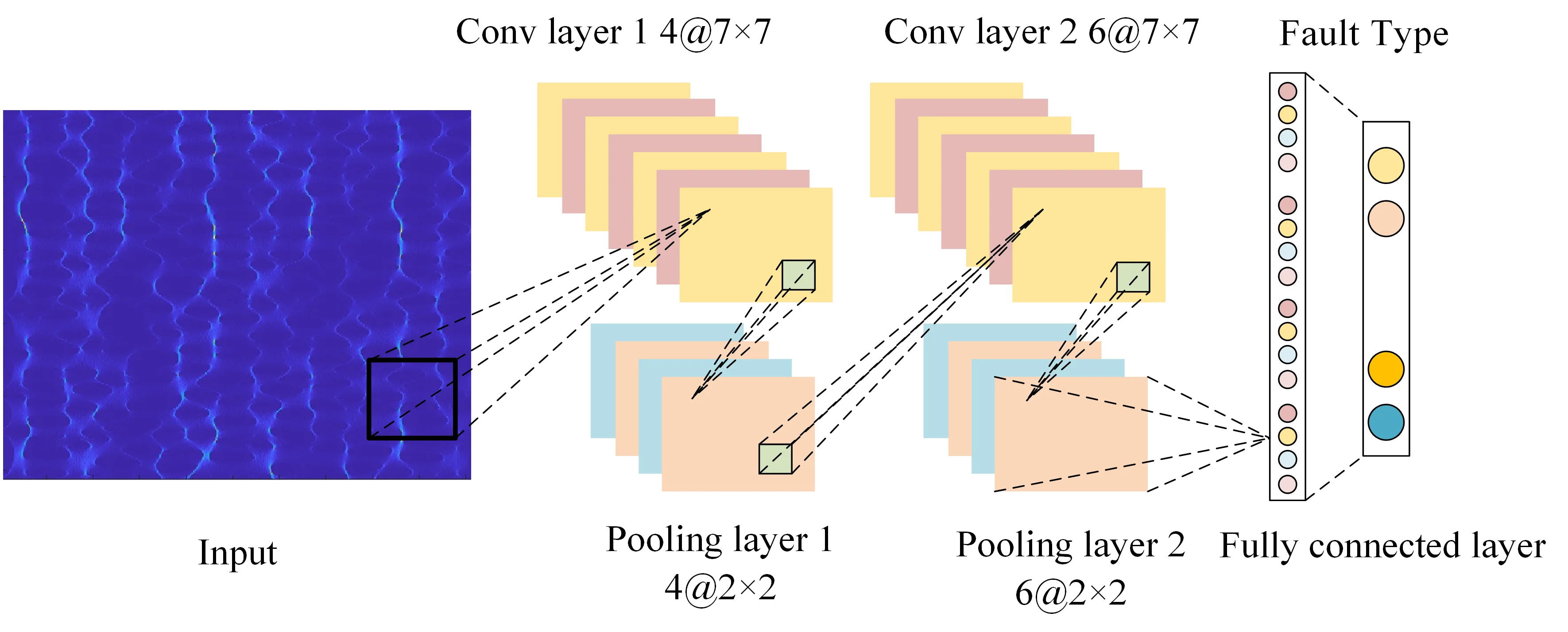
The ADAM optimization algorithm is employed to train the CNN, thereby optimizing the network parameters, specifically the weights and biases. ADAM's prowess lies in its ability to dynamically adjust the learning rate for each parameter by leveraging the first-order moment estimate (mean) and the second-order moment estimate (variance) of the gradient. This adaptive approach has been instrumental in enhancing the optimization process of CNN. Within the scope of this study, ADAM is utilized as both the feature extractor and classifier for the diagnosis of rolling bearing faults. To mitigate the risk of model overfitting, dropout operations are strategically incorporated into the FCL. The detailed architecture of the network is delineated in Table 1 and illustrated in Fig. 1.
Fig. 1The Structure of CNN
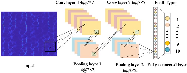
In Fig. 1, the input is a two-dimensional image. Firstly, four layers of convolution operations are performed to extract the features of the frequency domain image of the fault vibration signal. Then, the dimension is reduced through the pooling layer. After undergoing the above-mentioned convolution and pooling processes, all features are combined through the fully connected layer, and softmax is used to classify different features, thereby obtaining different bearing fault categories.
Table 1CNN structure parameters
Net layer | Conv kernel | Number of layers | |
C1 | Conv layer 1 | 7×7 | 4 |
P1 | Pooling layer 1 | 2×2 | 4 |
C2 | Conv layer 2 | 7×7 | 6 |
P2 | Pooling layer 2 | 2×2 | 6 |
F1 | Fully connected layer | 1×1 | 256 |
3.4. Reverse parameter update
For a specific classification task, the training objective of a CNN is to minimize the loss function of the network, thus it is crucial to select an appropriate loss function. Common loss functions include mean squared error, cross-entropy, and negative log-likelihood. In this paper, we choose the cross-entropy loss function, which has proven to be effective, and its expression is as follows Eq. (26):
where, represents the number of samples for a specific fault category; is the predicted value; and is the true value. During the training process, the method used to minimize the loss function is gradient descent. By taking the first-order partial derivative of Eq. (26), the learnable parameters ( and ) of the CNN can be updated layer by layer, as show in Eq. (27) and Eq. (28):
where, and represent the updated weights and biases, respectively; and are the current weights and biases; is the learning rate parameter, which controls the step size of weight updates. If is too large, it can cause the network to converge to a local optimum; if is too small, it will increase the training time of the network.
3.5. Reverse parameter update
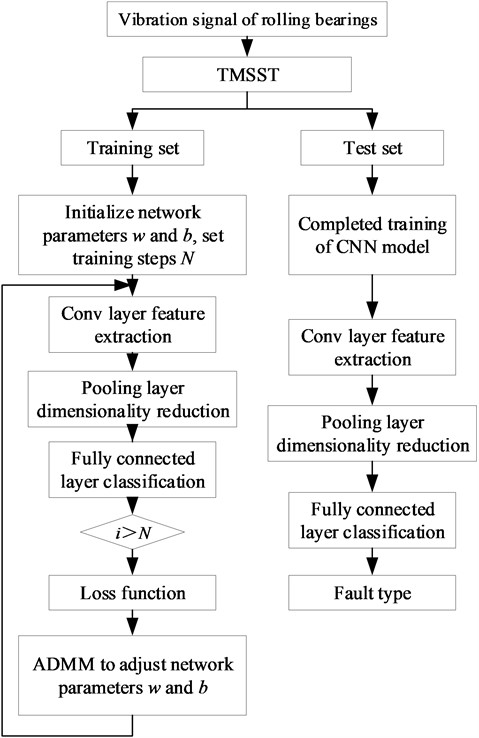
The fault diagnosis method based on CNN can integrate signal preprocessing, fault feature extraction, and fault pattern classification to achieve the specific process of adaptive extraction of fault features and intelligent diagnosis, as shown in Fig. 2. The collected vibration signals are divided into training and testing sets after TMSST. Firstly, the training set is input into the CNN for parameter learning, and the weights () and biases () are continuously updated using the gradient descent method. Then, the trained parameters are applied to the testing set to obtain the fault diagnosis results.
4. Experimental validation
This section aims to validate the feasibility and effectiveness of the proposed method using the measured vibration signals from rolling bearings. Furthermore, the robustness of the method under various fault conditions will be discussed.
Fig. 2Fault diagnosis flowchart based on TMSST-CNN
4.1. Dataset description
Fig. 3 shows the experimental platform, The testbed comprises a motor, torque sensor, power meter, and electronic controller. The bearing vibration signals are measured by sensors, and the amplitudes of these signals are represented by acceleration (https://engineering.case.edu/bearingdatacenter/apparatus-and-procedures).
To evaluate the performance of the proposed method, real bearing data were employed, which originated from the Bearing Fault Database of Case Western Reserve University [25]. This bearing fault database is a widely used resource that contains bearing vibration data under different operating conditions and fault modes, and is extensively employed in research on fault diagnosis and prediction. The testbed comprises a motor, torque sensor, power meter, and electronic controller. The bearing vibration signals are measured by sensors, and the amplitudes of these signals are represented by acceleration. The database includes both normal data and data from various fault modes, such as inner race faults, outer race faults, and rolling element faults. Each fault mode has multiple samples under different operating conditions, including varying parameters like rotational speed, load, and operating time. SKF's 6205-2RS deep groove ball bearing was taken as an example, and the drive-end bearing data were selected for verification. Single-point faults were arranged on the inner ring, outer ring, and rolling elements of the rolling bearing using electrical discharge machining techniques. Three fault diameters of 0.18, 0.36, and 0.54 mm were considered, with all faults having a depth of 0.28 mm. In total, nine fault types were examined. In this experiment, the length of each segment was determined to be 300 samples. 400 samples were constructed for each type of signal feature, and One-hot encoding was adopted to label ten different bearing operating conditions. The dataset was then divided into a training set and a test set in a 7:3 ratio. The construction of rolling bearing samples is summarized in Table 2. It includes ten different operating conditions, including normal state and nine different fault states, and the same proportion of data sets is taken.
Fig. 3Fault bearing vibration signal acquisition platform
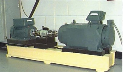
Table 2Sample structure of rolling bearing
Diameter (mm) | 0.17 | 0.36 | 0.54 | 0 | Load | ||||||
Rolling | Inner | Outer | Rolling | Inner | Outer | Rolling | Inner | Outer | Normal | ||
Label | 1 | 2 | 3 | 4 | 5 | 6 | 7 | 8 | 9 | 10 | |
Train | 280 | 280 | 280 | 280 | 280 | 280 | 280 | 280 | 280 | 280 | 0.746 kW |
Test | 120 | 120 | 120 | 120 | 120 | 120 | 120 | 120 | 120 | 120 | |
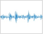
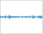
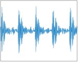
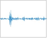
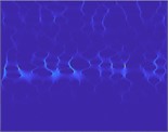
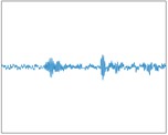
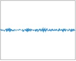
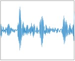
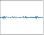
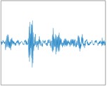
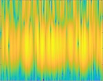
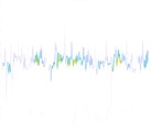
Fig. 4TMSST time-frequency diagrams for different types of faults: a) Normal; b) 0.17 mm rolling fault; c) 0.17 mm inner fault; d) 0.17 mm outer fault; e) 0.36 mm rolling fault; f) 0.36 mm inner fault; g) 0.36 mm outer fault; h) 0.54 mm rolling fault; i) 0.54 mm inner fault; j) 0.54 mm outer fault
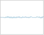

a) Normal

b) Fault 1
c) Fault 2

d) Fault 3

e) Fault 4

f) Fault 5

g) Fault 6

h) Fault 7

i) Fault 8

j) Fault 9
Traditional time-domain analysis has difficulties in accurately representing the damage severity and fault type characteristics of rolling bearings. Therefore, by leveraging the uniqueness of TMSST encoding in mapping time series, the original vibration signals are encoded to generate distinct fault patterns, as shown in Fig. 4. Subsequently, these patterns are classified using CNN for the identification of 10 types of rolling bearing features.
Fig. 4 presents the TMMST diagrams for ten distinct fault types. It is evident that traditional time-domain analysis of fault signals struggles to precisely articulate the extent of deterioration and the distinctive characteristics of various fault types in rolling bearings. Consequently, employing the time reassignment multi-synchronous compression transformation to convert the time-domain signals of rolling bearings into 2D time-frequency images can significantly amplify the discernible features of different fault types. As depicted in Fig. 4, signals characterized by dissimilar damage features and fault types are challenging to discern in the time domain, whereas 2D images are adept at effectively extracting their fault characteristics. Furthermore, this study conducts a comparative analysis of TMMST with several other signal processing techniques, including the STFT, HHT, WVD, Synchronous Compression Transform (SCT), Multiscale Synchronous Compression Transform (MS-SCT), Time-Reassigned Multisynchronous Compression Transform (TR-MS-SCT), and Time-Reassigned Synchronous Compression Transform (TR-SCT). For instance, in fault type 2, the corresponding 2D image is displayed in Fig. 5. Post these transformations, the CNN is integrated to classify the feature maps corresponding to the 10 types of faults.
Fig. 5Result chart of frequency domain variation methods for 0.17 mm inner fault at different times
a) STFT
b) HHT
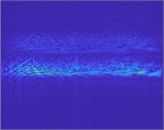
c) WVD

d) SST

e) MSST
4.2. Experimental result
To further verify the reliability of the proposed method, TMSST-CNN was used to identify ten types of faults in rolling bearings. There are a total of 4000 samples in the training and testing sets, divided into ten types of faults. In this section, the dataset was shuffled and the fault diagnosis model of TMMST-CNN was used to verify the model with different proportions of training and testing sets. The verification results are shown in Fig. 6.
From the confusion matrices presented in Figs. 5-6, it is evident that when the proportion of the training set is set to 70 %, a higher accuracy is achieved compared to when it is set to 60 %. Additionally, it can be effectively observed that the majority of misclassifications occur primarily in the categorization of Fault 6 and Fault 9. Examination of Fig. 4 reveals that the faults prone to misclassification exhibit insufficiently distinct characteristics in terms of energy distribution and varying fluctuation durations. However, upon undergoing the TMSST transformation, these differences become more prominent, resulting in a richer set of characteristics. To further validate the superiority of the method proposed in this study, a comparison was conducted between TMMST and other methods.
4.3. Experimental comparison
To verify the superiority of the proposed method, in this section, TMMST was compared with Short Time Fourier Transform, Hilbert Huang Transform, Wigner Ville Distribution, Synchronous Compression Transform, and Multiscale Synchronous Compression Transform. To highlight the superiority of TMSST-CNN, the accuracy, precision, and recall in the confusion matrix were used as evaluation indicators. Accuracy is the overall evaluation of the identification effect of all types of load appliances in the test set. The values of these evaluative metrics are bounded within the interval [0,1], where a higher value indicates superior identification capabilities of the algorithmic model [21]. These metrics are computed using the formulas presented in Eq. (29-32):
Fig. 6Performance of the method proposed in this article on different training sets: a) the accuracy of each type of fault when the training set is 60 %, b) the accuracy of each type of fault when the training set is 70 %
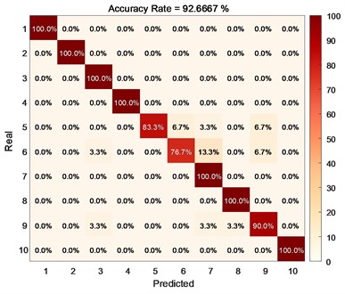
a)
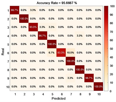
b)
In Table 3, represents the proportion of correctly predicted samples out of the total number of samples. In fault diagnosis, a high relative accuracy indicates that the model is able to reliably identify faulty and non-faulty states. is the proportion of actual positive samples (faulty state) among the predicted positive samples, reflecting the model’s ability to avoid misdiagnosing non-faulty states as faulty. , also known as recall, signifies the model's capability to capture the majority of faulty states, thereby reducing the risk of missed detections. The , on the other hand, provides a balanced consideration of both precision and recall, making it highly useful for evaluating the overall performance of the model in specific applications.
In the formula, represents the number of correctly classified fault types in the test set; represents the total number of fault types in the test set; is a true positive, representing the number of faults in this article where the predicted label of the fault type in the test set matches the true label; is a false negative, which represents the number of faults in the test set that were mistakenly identified as other types of faults for a certain type of fault; is false positive. In this article, it represents the number of faults in the test set that were incorrectly identified as a certain type of fault, while other types of faults were identified as such.
Through the analysis of Table 3, it can be seen that compared to directly using time-domain signals for evaluation in CNN models, time-frequency transformation can effectively improve the diagnostic rate of fault types. Meanwhile, compared to traditional time-frequency transformation methods, the method proposed in this paper has better performance. , , , and all have the best performance, with a global accuracy of 95.67 %. They have very high accuracy for 10 types of faults in rolling bearings and have a certain degree of robustness. Therefore, TMSST's processing of time-domain signals can effectively enhance data features, and TMSST-CNN is a method with a good diagnostic success rate for bearings.
Table 3Comparison results of different methods
CNN | STFT-CNN | HHT-CNN | WVD-CNN | SST-CNN | MSST-CNN | TMSST-CNN | |
85.92 % | 91.06 % | 88.32 % | 90.67 % | 93.21 % | 93.44 % | 95.67 % | |
86.44 % | 82.14 % | 89.28 % | 91.55 % | 93.94 % | 94.27 % | 96.34 % | |
86.06 % | 91.42 % | 89.10 % | 91.39 % | 93.88 | 94.02 % | 95.88 % | |
F -score | 87.33 | 92.74 | 91.02 | 92.61 | 95.35 | 96.12 | 98.12 |
5. Conclusions
This paper introduces a novel TMSST-CNN model for the diagnosis of rolling bearing faults. The TMSST component of the model takes into account the comprehensive integration of correlations across various time intervals during the encoding of rolling bearing signals. Consequently, when employed in conjunction with a CNN for the adaptive extraction of signal features and fault classification, it facilitates a more nuanced analysis, culminating in an impressive diagnostic accuracy of 95.67 %. To ascertain the model’s generalization capability, training was conducted using different ratios of training to testing data sets. The outcomes demonstrate that the model's performance has been markedly enhanced through the application of reinforcement learning techniques, consistently sustaining high diagnostic precision. A comparative analysis was undertaken across various image encoding methodologies and network architectures. The findings reveal that the TMSST image transformation technique outperforms alternative approaches in diagnosing rolling bearing faults. The methodology presented in this paper is capable of deeper learning, thereby attaining superior accuracy in fault diagnosis.
References
-
Y. Zhang, Z. Han, and D. Li, “Influence law of aerospace spur gear rim thickness on the tooth root stress,” (in Chinese), Machine Tool and Hydraulics, Vol. 48, No. 21, 2020.
-
Y. Zhang, “Analysis and prevention of gear transmission failure,” (in Chinese), Modern Rural Science and Technology, Vol. 33, No. 9, 2019.
-
Y. Zhang and R. B. Randall, “Rolling element bearing fault diagnosis based on the combination of genetic algorithms and fast kurtogram,” Mechanical Systems and Signal Processing, Vol. 23, No. 5, pp. 1509–1517, Jul. 2009, https://doi.org/10.1016/j.ymssp.2009.02.003
-
H. Wang, D. Xiong, Y. Duan, J. Liu, and X. Zhao, “Advances in vibration analysis and modeling of large rotating mechanical equipment in mining arena: A review,” AIP Advances, Vol. 13, No. 11, Nov. 2023, https://doi.org/10.1063/5.0179885
-
M. Kang, M. R. Islam, J. Kim, J.-M. Kim, and M. Pecht, “A hybrid feature selection scheme for reducing diagnostic performance deterioration caused by outliers in data-driven diagnostics,” IEEE Transactions on Industrial Electronics, Vol. 63, No. 5, pp. 3299–3310, May 2016, https://doi.org/10.1109/tie.2016.2527623
-
Q. Hu, X.-S. Si, A.-S. Qin, Y.-R. Lv, and Q.-H. Zhang, “Machinery fault diagnosis scheme using redefined dimensionless indicators and mRMR feature selection,” IEEE Access, Vol. 8, pp. 40313–40326, Jan. 2020, https://doi.org/10.1109/access.2020.2976832
-
J. Chen, C. Lu, and H. Yuan, “Bearing fault diagnosis based on active learning and random forest,” Vibroengineering PROCEDIA, Vol. 5, pp. 321–326, Jan. 2015.
-
D. Zhong, W. Guo, and D. He, “An intelligent fault diagnosis method based on STFT and convolutional neural network for bearings under variable working conditions,” in Prognostics and System Health Management Conference (PHM-Qingdao), Oct. 2019, https://doi.org/10.1109/phm-qingdao46334.2019.8943026
-
D. Verstraete, A. Ferrada, E. L. Droguett, V. Meruane, and M. Modarres, “Deep learning enabled fault diagnosis using time-frequency image analysis of rolling element bearings,” Shock and Vibration, Vol. 2017, pp. 1–17, Jan. 2017, https://doi.org/10.1155/2017/5067651
-
R. Yan, R. X. Gao, and X. Chen, “Wavelets for fault diagnosis of rotary machines: A review with applications,” Signal Processing, Vol. 96, pp. 1–15, Mar. 2014, https://doi.org/10.1016/j.sigpro.2013.04.015
-
V. Muralidharan and V. Sugumaran, “A comparative study of Naïve Bayes classifier and Bayes net classifier for fault diagnosis of monoblock centrifugal pump using wavelet analysis,” Applied Soft Computing, Vol. 12, No. 8, pp. 2023–2029, Aug. 2012, https://doi.org/10.1016/j.asoc.2012.03.021
-
J. Ben Ali, L. Saidi, A. Mouelhi, B. Chebel-Morello, and F. Fnaiech, “Linear feature selection and classification using PNN and SFAM neural networks for a nearly online diagnosis of bearing naturally progressing degradations,” Engineering Applications of Artificial Intelligence, Vol. 42, pp. 67–81, Jun. 2015, https://doi.org/10.1016/j.engappai.2015.03.013
-
J. Li, X. Yao, X. Wang, Q. Yu, and Y. Zhang, “Multiscale local features learning based on BP neural network for rolling bearing intelligent fault diagnosis,” Measurement, Vol. 153, p. 107419, Mar. 2020, https://doi.org/10.1016/j.measurement.2019.107419
-
Z. Huo, Y. Zhang, L. Shu, and M. Gallimore, “A new bearing fault diagnosis method based on fine-to-coarse multiscale permutation entropy, Laplacian score and SVM,” IEEE Access, Vol. 7, pp. 17050–17066, Jan. 2019, https://doi.org/10.1109/access.2019.2893497
-
X. Yan and M. Jia, “A novel optimized SVM classification algorithm with multi-domain feature and its application to fault diagnosis of rolling bearing,” Neurocomputing, Vol. 313, pp. 47–64, Nov. 2018, https://doi.org/10.1016/j.neucom.2018.05.002
-
Y. Li, Y. Yang, X. Wang, B. Liu, and X. Liang, “Early fault diagnosis of rolling bearings based on hierarchical symbol dynamic entropy and binary tree support vector machine,” Journal of Sound and Vibration, Vol. 428, pp. 72–86, Aug. 2018, https://doi.org/10.1016/j.jsv.2018.04.036
-
X. Zhang, Y. Liang, J. Zhou, and Y. Zang, “A novel bearing fault diagnosis model integrated permutation entropy, ensemble empirical mode decomposition and optimized SVM,” Measurement, Vol. 69, pp. 164–179, Jun. 2015, https://doi.org/10.1016/j.measurement.2015.03.017
-
J. Hou, X. Lu, Y. Zhong, W. He, D. Zhao, and F. Zhou, “A comprehensive review of mechanical fault diagnosis methods based on convolutional neural network,” Journal of Vibroengineering, Vol. 26, No. 1, pp. 44–65, Feb. 2024, https://doi.org/10.21595/jve.2023.23391
-
H. He, S. Zhao, W. Guo, Y. Wang, Z. Xing, and P. Wang, “Multi-fault recognition of gear based on wavelet image fusion and deep neural network,” AIP Advances, Vol. 11, No. 12, Dec. 2021, https://doi.org/10.1063/5.0066581
-
Z. Xing, Y. Liu, Q. Wang, and J. Li, “Multi-sensor signals with parallel attention convolutional neural network for bearing fault diagnosis,” AIP Advances, Vol. 12, No. 7, Jul. 2022, https://doi.org/10.1063/5.0095530
-
Z. Yuan, L. Zhang, L. Duan, and T. Li, “Intelligent fault diagnosis of rolling element bearings based on HHT and CNN,” in Prognostics and System Health Management Conference (PHM-Chongqing), pp. 292–296, Oct. 2018, https://doi.org/10.1109/phm-chongqing.2018.00056
-
X. Zheng, Y. Wei, J. Liu, and H. Jiang, “Multi-synchrosqueezing S-transform for fault diagnosis in rolling bearings,” Measurement Science and Technology, Vol. 32, No. 2, p. 025013, Feb. 2021, https://doi.org/10.1088/1361-6501/abb620
-
Y. Zhou, J. Chen, G. M. Dong, W. B. Xiao, and Z. Y. Wang, “Wigner-Ville distribution based on cyclic spectral density and the application in rolling element bearings diagnosis,” Proceedings of the Institution of Mechanical Engineers, Part C: Journal of Mechanical Engineering Science, Vol. 225, No. 12, pp. 2831–2847, Aug. 2011, https://doi.org/10.1177/0954406211413215
-
G. Yu, T. Lin, Z. Wang, and Y. Li, “Time-reassigned multisynchrosqueezing transform for bearing fault diagnosis of rotating machinery,” IEEE Transactions on Industrial Electronics, Vol. 68, No. 2, pp. 1486–1496, Feb. 2021, https://doi.org/10.1109/tie.2020.2970571
-
“Case Western Reserve University Bearing Data Center”, http://csegroups.case.edu/bearingdatacenter/pages/download-data-file.
About this article

The authors have not disclosed any funding.
The datasets generated during and/or analyzed during the current study are available from the corresponding author on reasonable request.
Yunxiu Zhang: conceptualization, methodology, formal analysis, writing-original draft, writing-review and editing, supervision. Bingxian Li: methodology, data collection, data analysis, resources, writing-review and editing. Zhiyin Han: literature review, conceptualization, writing-review and editing, visualization.
The authors declare that they have no conflict of interest.
