Abstract
The fault data for Planetary Roller Screw Mechanisms (PRSM) is challenging to collect in real industrial settings due to the complex nature of practical operations and the lengthy accumulation period. Consequently, there has been little research on PRSM fault diagnosis. Additionally, the high processing cost of PRSM means that institutions are reluctant to make their fault data publicly available, creating a data barrier and further hindering research of the study on fault diagnosis of PRSM. To address these issues, Federated Learning (FL) is applied for PRSM fault diagnosis. In the FL framework, data remains in local storage, preserving data privacy. To reduce transmission costs, a lightweight model called SResNet18 is proposed. SResNet18 reduces parameters by 95.07 % and 61.93 % compared to ResNet18 and DSResNet18, respectively, which decreases the time needed for parameter uploading, model aggregation, and parameter returning. Additionally, SResNet18 has lower computational complexity, with 92.09 % and 36.66 % fewer FLOPs than ResNet18 and DSResNet18, respectively. Healthy and fault data of PRSM are collected on the PRSM testing rig, and the proposed method is evaluated. Results show that our method achieves the highest accuracy of 99.17 %, improving model performance while maintaining data privacy. The proposed SResNet18 also alleviates overfitting and reduces training time in the FL framework.
Highlights
- Federated Learning (FL) is applied to PRSM fault diagnosis, ensuring data privacy and overcoming data barriers.
- SResNet18 significantly reduces model size and computational complexity, lowering transmission costs.
- SResNet18 achieves high accuracy while reducing overfitting and training time in the FL framework.
1. Introduction
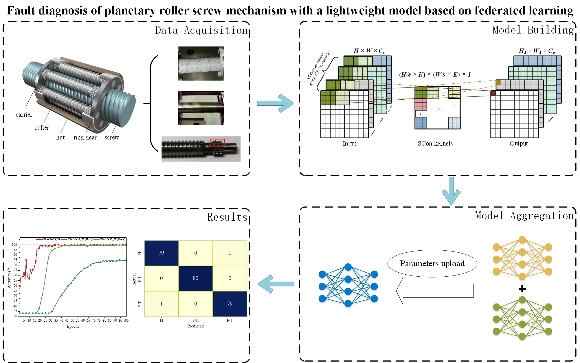
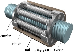
The Planetary Roller Screw Mechanism (PRSM) has become a preferred choice for electromechanical actuators due to its strong bearing capacity [1], high precision [2], and high limiting velocity [3]. The structure of the PRSM, illustrated in Fig. 1, primarily consists of carriers, a screw, rollers, a nut, and ring gears. Both the screw and nut have multi-start threads, while the roller has a single-start thread. Carriers at both ends support multiple rollers arranged uniformly around the circumference. The ends of the rollers are machined with spur gears that mesh with the ring gears fixed inside the nut.
Fig. 1Structure of PRSM
Currently, studies on PRSM primarily focus on load distribution [4]-[5], meshing principle and contact characteristic analysis [6]-[7] and dynamic characteristic analysis [8]-[9]. In recent years, the application of PRSM in aviation, aerospace, navigation and fields requiring precision servo transmission has gradually increased. However, PRSM typically operates with single redundancy, meaning its reliability directly impacts the reliability of the entire system. Therefore, there is an urgent need to develop effective fault diagnosis methods for PRSM.
However, most current fault diagnosis studies focus on gears, bearings and hydraulic pumps. For example, Huang et al. [10] and Sohaib et al. [11] proposed different fault diagnosis models to realize the fault diagnosis of gearboxes. Gu et al. [12] used modulation signal bispectrum and vibration measurements to diagnose gradual deterioration of gear. Zhao et al. [13] employed spatial decoupling method and the residual network for bearing fault diagnosis. Tao et al. [14] used the 18-layer residual neural network for bearing fault diagnosis, and compared it with SVM and LeNet. The results showed that the 18-layer residual neural network was better than SVM and LeNet. Zhao [15] utilized Depthwise Separable Convolution (DSC) for motor bearing fault diagnosis, showing shorter training times compared to VGG16, ResNet50, and MobileNetV3 without sacrificing accuracy. To reduce noise interference, Zhen et al. [16] used variational mode decomposition and degree of cyclostationarity demodulation to extract features of bearings. To solve class imbalance problems, Wu et al. [17] presented a deep adversarial transfer learning model. Cheng et al. [18] proposed a fault diagnosis model based on improved empirical wavelet transform-support vector machine for rolling bearing fault characteristics extraction and diagnosis. Mao et al. [19] developed a cross-domain feature extraction model and a bearing cross domain fault diagnosis model based on multi-layer perception mechanism to improve the accuracy of bearing cross domain fault diagnosis. Chao et al. [20] utilized a physical flow loss model and support vector data description model to assess the health status of hydraulic axial piston pumps. Yong et al. [21] applied Bayesian algorithm and improved CNN based on the S transform of multiple source signals for fault diagnosis of hydraulic axial piston pump. Tang et al. [22] used continuous wavelet transform, a lightweight model based on convolution and Bayesian algorithm for hydraulic axial piston pump failure recognition. The scarcity of fault diagnosis studies on PRSM is due to the complex and expensive processing technology compared to more mature technologies for gears and bearings. The price of a set of PRSM may be hundreds or thousands of times more than a set of gears. Additionally, there are numerous public datasets for bearing and gear faults, such as CWRU [23], XJTU-SY [24] and Gearbox Datasets [25]. For PRSM, Niu et al. [26] used a bird swarm algorithm and SVM to realize the fault diagnosis of PRSM, while Niu et al. [27] proposed a one-class model called deep Support Vector Data Description (deep SVDD) to determine whether PRSM is normal or not. However, these studies only consider a single type of PRSM failure. All the aforementioned methods require data to be aggregated in local storage, excluding data from other sources, which limits model training. In practice, data is often private, and collecting fault data is challenging with long accumulation periods. Consequently, few institutions make their data openly accessible, creating data barriers and leading to insufficient data for model training. Moreover, the model trained by data from one institution often perform poorly when applied to other institutions within the same field.
Based on the above analysis, breaking the data barrier between various institutions and making full use of multi-client data for model training is key to improving the performance of fault diagnosis models. To address these challenges, McMahan et al. [28] proposed Federated Learning (FL) in 2017. Currently, there are few studies on research of fault diagnosis based on FL. For instance, Chen et al. [29] used discrepancy-based weighted federated averaging to train the diagnosis model. Wang et al. [30] proposed an efficient asynchronous Federated Learning method to increase the efficiency of synchronization optimization. Zhang et al. [31] explored a Federated Learning model based on similarity collaboration to alleviate data heterogeneity for different conditions and fault diagnosis tasks. Liu et al. [32] addressed the domain shift issue with a federated transfer model based on broad learning. Yu et al. [33] introduced a new federated framework, FedCAE, for fault diagnosis to avoid potential conflicts arising from sharing data. Xue et al. [34] proposed a federated transfer learning method with consensus knowledge distillation and mutual information regularization to bridge the gap between source clients with labeled data and target clients without labeled data. However, these studies do not consider reducing transmission costs in the FL framework.
To address the lack of PRSM fault diagnosis data held by individual institutions and the absence of public PRSM datasets, FL is applied to train the model. The model is trained locally at each client without data communication, breaking the data barrier and improving the model performance. The vibration data in the , and direction of PRSM are not completely independent, indicating a relationship among three directions. However, as a time sequence signal, the signal at each time point differs significantly. Based on these vibration data characteristics and inspired by literature [35], a novel model with few parameters called SResNet18 is proposed to reduce the cost of parameter transmission. Experiments on the PRSM dataset is implemented, and the results show that the proposed method achieves the best effect. The main contributions and innovations of this paper are as follows:
1) Healthy and fault data of PRSM are collected on a PRSM testing rig, addressing the problem of insufficient PRSM fault data.
2) FL is applied for fault diagnosis of PRSM, solving the issue of limited studies on fault diagnosis of PRSM and there is no data communication among different institutions. In the FL framework, data barrier between different clients is broke. Combining data from various institutions enhances the performance of the fault diagnosis model.
3) To reduce the cost of parameter transmission in the FL framework, a lightweight model with few parameters, called SResNet18, is proposed.
The remainder of this paper is organized as follows. Section 2 details our method, including Federated Learning and lightweight model. Section 3 presents the experiments, results and discussion. Finally, conclusions are drawn in Section 4.
2. Fault diagnosis with a lightweight model based on Federated Learning
2.1. Framework of proposed method
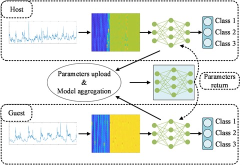
Fig. 2 shows the general implementation of the proposed method. In this study, two clients participate in training the model. To validate the effectiveness of FL, both clients process the data in the same way. In the FL framework, the training task is initiated by Guest and the model is built by Guest. Therefore, the models of Host and Guest are identical. At each round, Host and Guest upload parameters of the model, and then the model is aggregated. Finally, parameters of the global model are returned to each client. Through multiple training rounds, an optimized global model can be built.
Fig. 2Flow chart of the proposed method
2.2. Federated learning
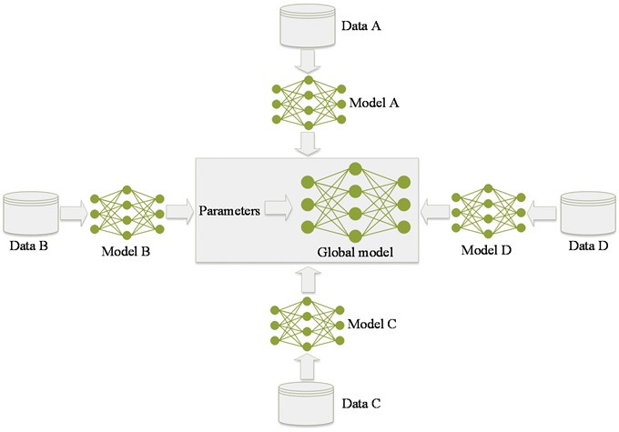
Traditional machine learning can only use data stored locally to train models, and the quantity and quality of data significantly impact model performance. Often, the data available in an institution’s local storage is insufficient to meet these requirements. Models with excellent performance typically require the aggregation of data from multiple clients. However, due to data privacy concerns, many institutions are reluctant to make their data publicly accessible.
To address this issue, FL is used for fault diagnosis. In the FL framework, data distributed across various institutions is utilized to train the model. Each client trains a model on its local data, and then uploads the model parameters. These parameters are exchanged among clients to aggregate the models, ultimately the global model is obtained. The implementation of FL is shown in Fig. 3. This approach allows each client to benefit from the data of other clients for model training while ensuring that the data remains within local storage.
Fig. 3Federated learning
The data of Host is , and the data of Guest is . These datasets do not overlap. A model with the same structure is built for both Host and Guest. The parameters of the models for Host and Guest are denoted as and , respectively. The outputs of the model for Host and Guest are calculated as follows:
where • represents computation involving the inputs and weights. In the FL framework, there are multiple Host clients, so the parameter represents the -th Host client.
The parameters of the global model are denoted , and the aggregation is implemented as follows:
where is the number of clients. In this way, parameters of Host and Guest are both .
The core idea of FL is that the data does not move, but the model does. Data remains local and is available but not visible to other clients. With this core idea, every client cooperates to build the model. This method preserves data privacy while making full use of multi-client data to collaboratively train the model.
2.3. Lightweight model
In the FL framework, parameters need to be continuously uploaded, aggregated and returned. Therefore, a model with a small number of parameters is necessary to reduce training time. The vibration data in the , and directions of PRSM is not completely independent, and there is a relationship among these directions. However, as a time sequence signal, the signal at each time point differs significantly. Based on the above characteristics of vibration data and inspired by literature [35], kernels with different weights should be used at different spatial positions, while kernels with same weights should be used across different channels. To achieve this, a novel layer called Symmetric Convolution (SConv) is proposed. and a new lightweight model with SConv as the main structure is built.
When extracting features on same channel, the kernels at different spatial positions are different. This allows for more accurate adaptive extraction of information at various spatial positions. All channels share one group of kernels, which significantly reduces number of parameters of the model. This design ensures efficient use of resources while maintaining the capability to capture important features. SConv can effectively extract features by applying large-size kernels to capture long-distance dependencies in the data.
For SConv, all channels of the input are treated as a group. SConv kernels are expressed as , where represents the size of the input, and represents the size of Sconv kernels. All channels share a group of SConv kernels with the same weights. The output of every channel is as follows:
where and refer to the input and kernel of the neighborhood on the center pixel. represents the -th channel.
The implementation flow of SConv is shown in Fig. 4.
Fig. 4Implementation flow of SConv
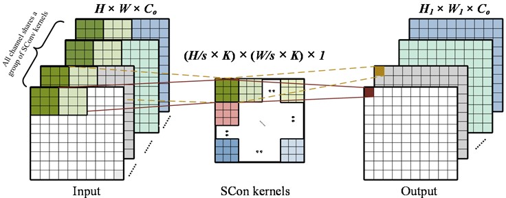
As shown in Fig. 4, the number of channels for both the input and output is . Therefore, a convolution layer with a kernel size of 1×1 and stride of 1 is usually needed to change the number of channels.
Since multiple SConv kernels with different weights are required at different spatial positions, it is necessary to dynamically generate different SConv kernels for these positions. In this paper, SConv kernels are generated through a bottleneck layer, as illustrated in Fig. 5.
Fig. 5The implementation of SConv kernels generation
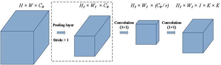
As shown in Fig. 5, the parameter determines the size of the bottleneck layer. When the stride is not equal to 1, the height and width of the input will change. Consequently, the size of the SConv kernels generated through a single bottleneck layer may not match the input size. To address this, a pooling layer is used to reduce the height and width of the input. After the pooling layer, the height and width of the input become and , respectively. When the stride is equal to 1, the size of the kernels generated through the bottleneck layer matches the input size input, within the dotted line in Fig. 5 is not required.
2.4. The architecture of SResNet18
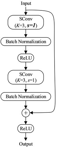
When training the model in the FL framework, the training time of the fault diagnosis model is mainly composed of two parts. The first part is the time spent training the model locally, and the second part is the time taken to upload the model parameters, aggregate the models from all clients, and return the global model parameters to all clients. Therefore, reducing the complexity of the model can not only decrease the computational cost but also reduce local training time. It is also crucial to reduce the number of model parameters. Fewer parameters lower transmission costs, thus reducing the overall training time. To achieve this, the convolution layers in ResNet18 [36] are replaced with SConv layers. In this way, SResNet18 is built for fault diagnosis of PRSM. The overall structure is shown in Fig. 6. SRes1 and SRes2 are shown in Fig. 7.
Fig. 6The structure of SResNet18
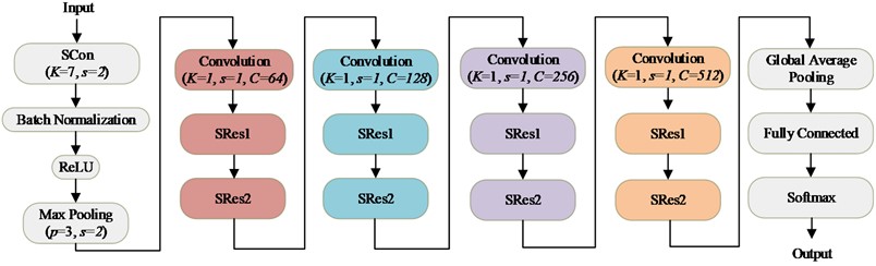
As shown in Fig. 6, In addition to the traditional ResNet18 structure, there are four additional convolution layers with the kernel size of 1×1 and the stride of 1. These four convolution layers are designed to change the number of output channels.
Fig. 7The structure of SRes
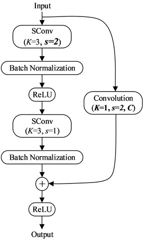
a) SRes1
b) SRes2
3. Experiments, results and discussion
3.1. The description of datasets
3.1.1. Data collection
The PRSM testing rig is shown in Fig. 8, which includes servo motor, coupling, tested PRSM, accelerometer and hydraulic loading system.
Fig. 8PRSM testing rig
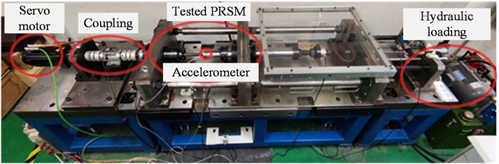
Fig. 9 shows the healthy (H), failure of lubrication (F-L) and failure of the teeth on one side of the roller (F-T).
The nominal diameter of the tested screw is 24 millimeters. The pitch is 2 millimeters and the number of rollers is 10. Due to the limited effective travel, the screw cannot continuously rotate in the same direction. Therefore, the screw operates in a forward and reverse motion, and the nut reciprocates linearly. Except for the reversing stage, the linear velocity of the nut remains constant. The load differs when the nut extends and retracts, resulting in load fluctuations within a certain range. The given load is the maximum load of the actual load. In this paper, rotating speed of 104 r/min is implemented, and the load is 9 kN. An accelerometer is installed on the nut to collect the vibration signals in the , and direction with a sampling frequency of 20 kHz.
Fig. 9The different states of PRSM
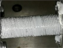
a) H
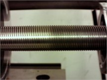
b) F-L
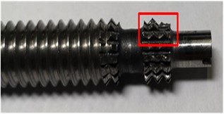
c) F-T
3.1.2. Data process
In this paper, there are two clients training the model: Host and Guest. The raw data is randomly divided between Host and Guest to simulate the real industrial scenario, where each client’s training set is non-overlapping and the data is unevenly distributed.
The data is normalized according to Eq. (4) to reduce the data span. Since acceleration data has directionality, the collected data includes both positive and negative values. To preserve this directionality, the data is normalized to the range [–1, 1]:
where represents the input. and represent the maximum and minimum value of normalized data and they are set to 1 and –1 respectively. Then the normalized data is enhanced by window clipping and is processed using wavelet packet transform.
The final datasets are described Table 1.
Table 1Description of datasets
Datasets | Client | Class | Samples | Label | One-hot |
Training | Host | N | 252 | 0 | [0 0 1] |
F-L | 252 | 1 | [0 1 0] | ||
F-T | 252 | 2 | [1 0 0] | ||
Guest | N | 349 | 0 | [0 0 1] | |
F-L | 349 | 1 | [0 1 0] | ||
F-T | 349 | 2 | [1 0 0] | ||
Testing | Host and guest | N | 80 | 0 | [0 0 1] |
F-L | 80 | 1 | [0 1 0] | ||
F-T | 80 | 2 | [1 0 0] |
For each state, there are 252 and 349 samples for Host and Guest, respectively, with label values of 0, 1, and 2. The testing set contains 80 samples for each state. To compare the performance of the FL model and single-point (SP) model, which is trained using the local data of a single client, the testing set is shared.
3.2. Comparison models and experimental setup
As previously mentioned, the fault diagnosis performance of the 18-layer convolution residual neural network (ResNet18) proposed by Tao et al. [14] is superior to that of SVM and LeNet. The performance of the model based on DSC proposed by Zhao [15] outperforms VGG16, ResNet50 and MobileNetV3. Therefore, this paper compares the proposed model with ResNet18 and 18 layer depth wise separable convolution (DSResNet18).
In this paper, kubefate-docker-compose-v1.6.0 is chosen as the FL framework. which only supports CPU. The model is trained using an Intel (R) Core (TM) i5-5200U CPU for the Host and an Intel (R) Core (TM) i5-10200H CPU for the Guest. Adam is used as the optimizer. The batch size, number of training epochs and learning rate are set to 64, 100 and 0.01 respectively.
3.3. Results and discussions
To evaluate the performance of FL model as well as the impact of the number of parameters and model complexity on the federated training speed, this section will assess the performance of each model during the model training and testing respectively.
3.3.1. Parameters, FLOPs and training time
Parameters, FLOPs and training time of SP model and FL model are shown in Table 2.
Table 2Parameters, FLOPs and training time
Model | Parameters / M | FLOPs / G | Training time (SP) / s | Training time (FL) / s |
ResNet18 | 11.2 | 0.297 | 977 | 9039 |
DSResNet18 | 1.45 | 0.0371 | 284 | 1836 |
SResNet18 | 0.552 | 0.0235 | 650 | 3551 |
In this paper, SP models are trained three times. The training time shown in Table 2 for SP models refers to the model with the highest accuracy. Due to the longer training time and higher cost for FL models, they are only trained once. As shown in Table 2, the number of parameters and FLOPs of DSResNet18 and SResNet18 are significantly fewer than those of ResNet18. with SResNet18 being the least. However, despite the number of parameters and FLOPs are the least, training time for both SP model and FL model are not the shortest. One possible reason is that SResNet18 includes four additional convolution layers with a kernel size of 1×1 and stride of 1. Additionally, the implementation of SConv requires to generate kernels through the bottleneck layer, followed by multiplication and addition with the input, making the computation process more complex than DSC. The sequential nature of kernel generation and subsequent multiplication and addition prevents parallel implementation. Another reason is that existing hardware devices are more optimized for mature neural networks like CNN and DSC. Thus, when the difference in number of parameters and FLOPs is slight, the training speed of mature neural networks tends to be faster than that of the newly proposed one. Training time for SP model is shorter than that for FL model, with a significant difference between the two. In the FL framework, training time includes parameters uploading, model aggregation, and parameters returning, which constitute a large proportion of the total time. Additionally, when multiple clients participate in training the model, the overall training speed is often limited by the performance of the least powerful computer.
3.3.2. Convergence speed on training set
In the FL framework, the training task is initiated by Guest. To compare the convergence speed and accuracy of SP model and FL model on training set, Fig. 10 presents accuracy on training set of ResNet18, DSResNet18, SResNet18 SP model and FL model. SP models shown in Fig. 11 refer to the model with the highest accuracy.
The conclusions drawn from Fig. 10 are as follows:
1) SP model converges faster than FL model for each client. This is because FL model not only needs to extract the features from one client’s data, but also from the other client's unseen data. When extracting features from another client’s unseen data, the model parameters are not directly obtained from the data but are averaged from the parameters of both models. This averaging process can sometimes misalign with the feature distribution of each client. Adjusting the model parameters can also disrupt the locally extracted features or diverge from the intended convergence direction.
2) The accuracy on the training set for Guest is higher than that of Host. The possible reason is that Guest holds more data, enabling the model trained by Guest to extract more features. After model aggregation, the global model achieves better fit on the data of Guest.
Fig. 10Accuracy on training set of different models
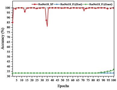
a) ResNet18
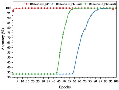
b) DSResNet18
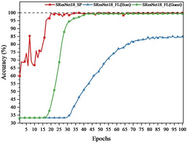
c) SResNet18
3.3.3. Accuracy on training set and testing set
Accuracy on training set of SP model and FL model in the stable stage, as well as accuracy on testing set, are shown in Table 3.
Table 3Accuracy of SP model and FL model
Model | Accuracy of SP model | Accuracy of FL model | |||
Training | Testing | Training (Host) | Training (Guest) | Testing | |
ResNet18 | 99.92 %±0.09 | 66.97 %±0.46 | 33.33 % | 37.06 % | 36.25 % |
DSResNet18 | 99.78 %±0.20 | 96.11 %±1.58 | 100.00 % | 100.00 % | 97.92 % |
SResNet18 | 99.75 %±0.29 | 98.19 %±0.64 | 84.92 % | 99.43 % | 99.17 % |
As mentioned above, SP models are trained three times, and the mean and standard deviation of the accuracy on training set and testing set are provided in Table 3, while the FL models are only trained once due to its high training cost and time. In the FL framework, accuracy on testing set for the models may be higher than accuracy on training set of Host, but it is lower than accuracy on training set of Guest. The possible reason is that Host holds less data, resulting in weaker feature extraction by the model. Therefore, the global model aligns more closely with Guest's feature distribution than with Host’s. For SP model, accuracy on testing set is lower than accuracy on training set, indicating that there are different degrees of overfitting among the models, with ResNet18 showing the most significant overfitting. This is likely due to an insufficient number of samples for single-point training, which doesn’t match the model's large number of parameters. The standard deviation provided in Table 3 reflects the uncertainty in model accuracy. For instance, the ResNet18 SP model has a higher uncertainty (standard deviation of ±0.46) compared to SResNet18 (±0.64), indicating greater variability in its performance. Moreover, ResNet18 SP model achieves the highest accuracy on training set but the lowest accuracy on testing set. This indicates that ResNet18 SP model has poor generalization ability on new datasets and exhibits the highest uncertainty. In the FL framework, except for ResNet18, overfitting has been significantly alleviated for each model. This may be because the large number of parameters for ResNet18 means the number of training epochs does not meet the convergence requirements for the global model in the FL framework. However, increasing the number of epochs would raise the training time and computational cost, leading to unnecessary waste. As shown in Table 3, compared to SP model, FL model shows a slighter difference between accuracy on testing set and accuracy on Guest’s training set, indicating that FL can alleviate overfitting caused by insufficient data.
To observe the results on testing set for FL model more intuitively, visualizations and confusion matrices of each model are as follows.
Based on the provided confusion matrices in Fig. 11, ResNet18 FL model performs the worst. There is no clear classification boundary among the samples of three states, and the samples are mixed together. While it achieves very high accuracy in predicting state H, it struggles significantly with predicting state F-L, resulting in higher uncertainty for state F-L. The sensitivity of the ResNet18 FL model is best for state H but varies significantly for state F-L and state F-H. Due to the large performance discrepancies across different states, the confidence interval for this model is likely wider, and its specificity is high for state H but lower for state F-L and F-H. In contrast, DSResNet18 FL model shows a more balanced performance across all states, with high prediction accuracy for state H, state F-L, and state F-H. This indicates lower uncertainty, high sensitivity and specificity, as well as a narrower confidence interval. SResNet18 FL model demonstrates the most stable performance, with high accuracy across all states. It can correctly classify the samples of each state, with a clear boundary among the samples of the three classes. Its uncertainty and confidence interval are both low, and it exhibits excellent specificity as it accurately identifies state H, state F-L and F-H. In summary, SResNet18 FL model performs the best overall, while ResNet18 FL model shows the most instability.
3.3.4. Model comprehensive performance
To clearly compare the performance of SP model and FL model, all the results are shown in Table 4.
As indicated in Table 4, SResNet18 SP model achieves the highest accuracy of 99.17 %. Although training time of DSResNet18 is the shortest, the accuracy of model on testing set is most crucial indicator when training time is close. With the highest accuracy on testing set, training time of SResNet18 is relatively short. In summary, the proposed SResNet18 FL model demonstrates the best performance.
Table 4Comparison results of model comprehensive performance
Model | Parameters / M | FLOPs / G | Accuracy on testing set | Training time / s | ||
SP model | FL model | SP model | FL model | |||
ResNet18 | 11.2 | 0.297 | 66.97 %±0.46 | 36.25 % | 977 | 9039 |
DSResNet18 | 1.45 | 0.0371 | 96.11 %±1.58 | 97.92 % | 284 | 1836 |
SResNet18 | 0.552 | 0.0235 | 98.19 %±0.64 | 99.17 % | 650 | 3551 |
Fig. 11The visualizations of the result and confusion matrix of different models
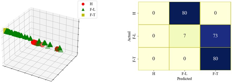
a) ResNet18
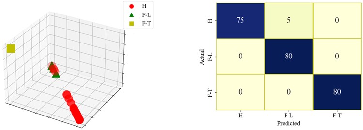
b) DSResNet18
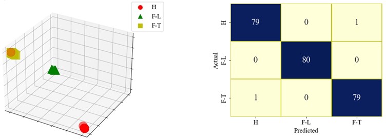
c) SResNet18
4. Conclusions
Given the challenges of collecting PRSM fault data in real industries, the long data accumulation period, data privacy concerns preventing communication between different institutions, and the scarcity of studies on PRSM fault diagnosis, this paper collects healthy and fault data of PRSM and applies FL to train the fault diagnosis model. To reduce transmission costs in the FL framework, a model called SResNet18 with fewer parameters and FLOPs is developed. Compared to ResNet18 and DSResNet18, SResNet18 has 95.1 % and 61.9 % fewer parameters, and 92.1 % and 36.7 % lower FLOPs, respectively. With healthy and fault data collected on the PRSM testing rig, the data is processed and the diagnosis experiment is conducted. The results show that the proposed SResNet18 FL model achieves the best performance, with faster convergence speed and the highest accuracy, reaching 99.2 %. Furthermore, FL enhances the model's performance and mitigates overfitting by learning from more samples while maintaining data privacy. For SResNet18, the FL model's accuracy increased by 8.0 % compared to the SP model. However, this study has its limitations. The training time for SResNet18 is longer than that of DSResNet18, this is because the implementation of SConv needs to generate kernels through the bottleneck layer, and then multiplication and addition with the input is implemented. To further reduce training time, future improvements should focus on enhancing the kernel generation process.
References
-
L. M. Yu, “Technical improvement and development of all-electric aircraft,” (in Chinese), Aircraft Design, Vol. 3, 1999, https://doi.org/10.19555/j.cnki.1673-4599.1999.03.001
-
R. Qi, H. Lin, and S. Y. Zhou, “Study on key techniques for electrical system of more-electric,” (in Chinese), Aeronautical Computing Technique, Vol. 34, No. 1, pp. 97–101, 2004, https://doi.org/10.3969/j.issn.1671-654x.2004.01.028
-
J. A. Rosero, J. A. Ortega, E. Aldabas, and L. Romeral, “Moving towards a more electric aircraft,” IEEE Aerospace and Electronic Systems Magazine, Vol. 22, No. 3, pp. 3–9, Mar. 2007, https://doi.org/10.1109/maes.2007.340500
-
L. Li, Y. Fu, S. Zheng, J. Fu, and T. Xia, “Friction torque analysis of planetary roller screw mechanism in roller jamming,” Mathematical Problems in Engineering, Vol. 2020, pp. 1–8, Mar. 2020, https://doi.org/10.1155/2020/1392380
-
Z. C. Gu, “Research progress of Power-By-Wire actuation technology,” (in Chinese), Science and Technology Vision, Vol. 5, pp. 141–175, 2017, https://doi.org/10.19694/j.cnki.issn2095-2457.2017.05.091
-
Y. Liu, J. Wang, H. Cheng, and Y. Sun, “Kinematics analysis of the roller screw based on the accuracy of meshing point calculation,” Mathematical Problems in Engineering, Vol. 2015, pp. 1–10, Jan. 2015, https://doi.org/10.1155/2015/303972
-
W. Shui-Ming, X. Qiang, L. Zhi-Wen, H. Yu-Ping, and P. Li-Ping, “Effect of profile error on meshing state of planetary roller screw,” in Chinese Automation Congress (CAC), pp. 20–22, Oct. 2017, https://doi.org/10.1109/cac.2017.8244129
-
X. Fu, G. Liu, R. Tong, S. Ma, and T. C. Lim, “A nonlinear six degrees of freedom dynamic model of planetary roller screw mechanism,” Mechanism and Machine Theory, Vol. 119, pp. 22–36, Jan. 2018, https://doi.org/10.1016/j.mechmachtheory.2017.08.014
-
Y. Li, “Redundant controller design for electric actuating cylinder of small aerial vehicle landing gear,” (in Chinese), Nanjing University of Aeronautics and Astronautics Press, Nanjing, 2016.
-
X. Huang, Y. Li, and Y. Chai, “Intelligent fault diagnosis method of wind turbines planetary gearboxes based on a multi-scale dense fusion network,” Frontiers in Energy Research, Vol. 9, p. 74762, Nov. 2021, https://doi.org/10.3389/fenrg.2021.747622
-
M. Sohaib et al., “Gearbox fault diagnosis using improved feature representation and multitask learning,” Frontiers in Energy Research, Vol. 10, p. 99876, Sep. 2022, https://doi.org/10.3389/fenrg.2022.998760
-
J. X. Gu, A. Albarbar, X. Sun, A. M. Ahmaida, F. Gu, and A. D. Ball, “Monitoring and diagnosing the natural deterioration of multi-stage helical gearboxes based on modulation signal bispectrum analysis of vibrations,” International Journal of Hydromechatronics, Vol. 1, No. 1, pp. 309–330, Jan. 2021, https://doi.org/10.1504/ijhm.2021.10040778
-
Y. Zhao, M. Zhou, X. Xu, and N. Zhang, “Fault diagnosis of rolling bearings with noise signal based on modified kernel principal component analysis and DC‐ResNet,” CAAI Transactions on Intelligence Technology, Vol. 8, No. 3, pp. 1014–1028, Jan. 2023, https://doi.org/10.1049/cit2.12173
-
Q. Tao, C. Peng, J. Man, and Y. Liu, “Two-step transfer learning method for bearing fault diagnosis,” (in Chinese), Computer Engineering and Applications, Vol. 58, No. 2, pp. 303–312, 2022, https://doi.org/10.3778/j.issn.1002-8331.2009-0207
-
C. Zhao, “Research on fault diagnosis method based on deep learning and image processing,” Shenyang Ligong University Press, Shenyang, 2021.
-
D. Zhen, D. Li, G. Feng, H. Zhang, and F. Gu, “Rolling bearing fault diagnosis based on VMD reconstruction and DCS demodulation,” International Journal of Hydromechatronics, Vol. 5, No. 3, p. 205, Jan. 2022, https://doi.org/10.1504/ijhm.2022.125092
-
Z. Wu, H. Zhang, J. Guo, Y. Ji, and M. Pecht, “Imbalanced bearing fault diagnosis under variant working conditions using cost-sensitive deep domain adaptation network,” Expert Systems with Applications, Vol. 193, p. 116459, May 2022, https://doi.org/10.1016/j.eswa.2021.116459
-
Z. Cheng, “Extraction and diagnosis of rolling bearing fault signals based on improved wavelet transform,” Journal of Measurements in Engineering, Vol. 11, No. 4, pp. 420–436, Dec. 2023, https://doi.org/10.21595/jme.2023.23442
-
X. Mao, “Cross domain fault diagnosis method based on MLP-mixer network,” Journal of Measurements in Engineering, Vol. 11, No. 4, pp. 453–466, Dec. 2023, https://doi.org/10.21595/jme.2023.23460
-
Q. Chao, Z. Xu, Y. Shao, J. Tao, C. Liu, and S. Ding, “Hybrid model-driven and data-driven approach for the health assessment of axial piston pumps,” International Journal of Hydromechatronics, Vol. 6, No. 1, p. 76, Jan. 2023, https://doi.org/10.1504/ijhm.2023.129123
-
Y. Zhu, S. Tang, and S. Yuan, “Multiple-signal defect identification of hydraulic pump using an adaptive normalized model and S transform,” Engineering Applications of Artificial Intelligence, Vol. 124, p. 106548, Sep. 2023, https://doi.org/10.1016/j.engappai.2023.106548
-
S. Tang, B. Cheong Khoo, Y. Zhu, K. Meng Lim, and S. Yuan, “A light deep adaptive framework toward fault diagnosis of a hydraulic piston pump,” Applied Acoustics, Vol. 217, p. 109807, Feb. 2024, https://doi.org/10.1016/j.apacoust.2023.109807
-
W. A. Smith and R. B. Randall, “Rolling element bearing diagnostics using the Case Western Reserve University data: a benchmark study,” Mechanical Systems and Signal Processing, Vol. 64-65, pp. 100–131, Dec. 2015, https://doi.org/10.1016/j.ymssp.2015.04.021
-
L. Yaguo, H. Tianyu, W. Biao, L. Naipeng, Y. Tao, and Y. Jun, “XJTU-SY rolling element bearing accelerated life test datasets: a tutorial,” Journal of Mechanical Engineering, Vol. 55, No. 16, pp. 1–6, Jan. 2019, https://doi.org/10.3901/jme.2019.16.001
-
P. Cao, S. Zhang, and J. Tang, “Preprocessing-free gear fault diagnosis using small datasets with deep convolutional neural network-based transfer learning,” IEEE Access, Vol. 6, pp. 26241–26253, Jan. 2018, https://doi.org/10.1109/access.2018.2837621
-
M. Niu, S. Ma, W. Cai, J. Zhang, and G. Liu, “Fault diagnosis of planetary roller screw mechanism based on bird swarm algorithm and support vector machine,” in Journal of Physics: Conference Series, Vol. 1519, No. 1, p. 012007, Apr. 2020, https://doi.org/10.1088/1742-6596/1519/1/012007
-
M. Niu, S. Ma, W. Cai, J. Zhang, and W. Deng, “Fault diagnosis of planetary roller screw mechanism through one-class method,” (in Chinese), Journal of Chongqing University of Technology (Natural Science), Vol. 37, No. 2, pp. 307–315, 2023, https://doi.org/10.3969/j.issn.1674-8425(z).2023.02.034
-
H. B. Mcmahan, E. Moore, D. Ramage, S. Hampson, and B. A. Y. Arcas, “Communication-efficient learning of deep networks from decentralized data,” Proceedings of the 20th International Conference on Artificial Intelligence and Statistics (AISTATS), Vol. 54, pp. 1273–1282, Jan. 2016, https://doi.org/10.48550/arxiv.1602.05629
-
J. Chen, J. Li, R. Huang, K. Yue, Z. Chen, and W. Li, “Federated transfer learning for bearing fault diagnosis with discrepancy-based weighted federated averaging,” IEEE Transactions on Instrumentation and Measurement, Vol. 71, pp. 1–11, Jan. 2022, https://doi.org/10.1109/tim.2022.3180417
-
Q. Wang, Q. Li, K. Wang, H. Wang, and P. Zeng, “Efficient federated learning for fault diagnosis in industrial cloud-edge computing,” Computing, Vol. 103, No. 10, pp. 2319–2337, Jun. 2021, https://doi.org/10.1007/s00607-021-00970-6
-
Y. Zhang, X. Xue, X. Zhao, and L. Wang, “Federated learning for intelligent fault diagnosis based on similarity collaboration,” Measurement Science and Technology, Vol. 34, No. 4, p. 045103, Apr. 2023, https://doi.org/10.1088/1361-6501/acab22
-
G. Liu, W. Shen, L. Gao, and A. Kusiak, “Active federated transfer algorithm based on broad learning for fault diagnosis,” Measurement, Vol. 208, p. 112452, Feb. 2023, https://doi.org/10.1016/j.measurement.2023.112452
-
Y. Yu, L. Guo, H. Gao, Y. He, Z. You, and A. Duan, “FedCAE: A new federated learning framework for edge-cloud collaboration based machine fault diagnosis,” IEEE Transactions on Industrial Electronics, Vol. 71, No. 4, pp. 4108–4119, Apr. 2024, https://doi.org/10.1109/tie.2023.3273272
-
X. Xue, X. Zhao, Y. Zhang, M. Ma, C. Bu, and P. Peng, “Federated transfer learning with consensus knowledge distillation for intelligent fault diagnosis under data privacy preserving,” Measurement Science and Technology, Vol. 35, No. 1, p. 015108, Jan. 2024, https://doi.org/10.1088/1361-6501/acf77d
-
D. Li et al., “Involution: inverting the inherence of convolution for visual recognition,” in 2021 IEEE/CVF Conference on Computer Vision and Pattern Recognition (CVPR), pp. 12321–12330, Jun. 2021, https://doi.org/10.1109/cvpr46437.2021.01214
-
K. He, X. Zhang, S. Ren, and J. Sun, “Deep residual learning for image recognition,” in 2016 IEEE Conference on Computer Vision and Pattern Recognition (CVPR), pp. 770–778, Jun. 2016, https://doi.org/10.1109/cvpr.2016.90
About this article

The research is supported by Shaanxi Engineering Laboratory for Transmissions and Controls.
The datasets generated during and/or analyzed during the current study are available from the corresponding author on reasonable request.
Maodong Niu: methodology, software and writing-original draft preparation, writing-review and editing. Shangjun Ma: conception, methodology, data curation, project administration, writing-original draft preparation and writing-review and editing. Qiangqiang Huang and Pan Deng: software, writing-original draft preparation.
The authors declare that they have no conflict of interest.
