An effective simulation scheme for the prediction of aerodynamic environment under hypersonic conditions characterized by NACA0012

Ding, Fangli; Yang, Lu

doi:10.21595/jve.2024.24084

Journal of Vibroengineering

Browse Journal

Submit article

Published: 01 August 2024

Check for updates

An effective simulation scheme for the prediction of aerodynamic environment under hypersonic conditions characterized by NACA0012

Fangli Ding¹

Lu Yang²

¹College of Electrical Engineering, Tongling University, Tongling, China

²Department of Public Security Science and Technology, Anhui Public Security College, Hefei, China

Corresponding Author:

Lu Yang

Cite the article Download PDF

Article in Press

Downloads 0

Abstract

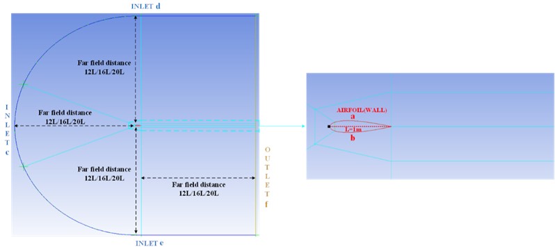
Currently, aerodynamic environment prediction research into scramjet-propelled vehicles characterized by NACA0012 under hypersonic conditions is relatively sparse. Two-dimensional external flow field models are established, and then through validation tests, we perform a systematic investigation between simulation parameters and prediction accuracy, and an effective aerodynamic environment prediction simulation scheme under hypersonic conditions is proposed. Unlike under incompressible conditions, the maximum accuracy decline could be attributed to the inappropriate choice of the sharp trailing edge modeling method, but the definition formula is still preferred. In particular, for the two modeling data point sources, Airfoil tools and NACA4, the numerical performance of the latter is better than the former, and the calculation accuracy negatively correlates with the number of data points offered by both of them. Moreover, for the mesh cells near the shock, the cell Reynolds number and aspect ratio values should be no smaller than 16 and not exceed 380, respectively, and the recommended values for the far field distance, the turbulence model and flux type are 16L, Spalart-Allmaras, and ROE flux type. Under hypersonic conditions, the aerodynamic environment characterized by NACA0012 predicts a maximum temperature of approximately 1856.85 °C, with an average temperature change rate of 77 °C/s. Meanwhile, the top sound pressure level and the vibration acceleration could reach up to 145 dB and 182 g, respectively.

1. Introduction

Adapting to the environment becomes crucial as the hypersonic vehicle encounters increasingly harsh flight conditions. NASA has identified environmental failure as the leading cause of previous vehicle launch crashes, emphasizing the criticality of environment testing. Therefore, it is imperative to first predict the aerodynamic environment experienced by the hypersonic vehicle and subsequently design its structure accordingly. By conducting comprehensive environment testing, potential issues can be identified and addressed to enhance flights’ reliability and adaptability in diverse environments. The predicted results of the aerodynamic environment serve as a fundamental basis for both vehicle design and subsequent environment testing. The accurate prediction of the aerodynamic environment is crucial for the design and optimization of the hypersonic vehicle. The main types of hypersonic vehicle include the ground-to-orbit reentry, the low-orbit reentry and the scramjet-propelled [1] and the reusable reentry vehicle is the leading research object [2]-[7], while the prediction research for the scramjet-propelled vehicle is relatively sparse. Hence, we focus our research on the scramjet-propelled hypersonic vehicle.

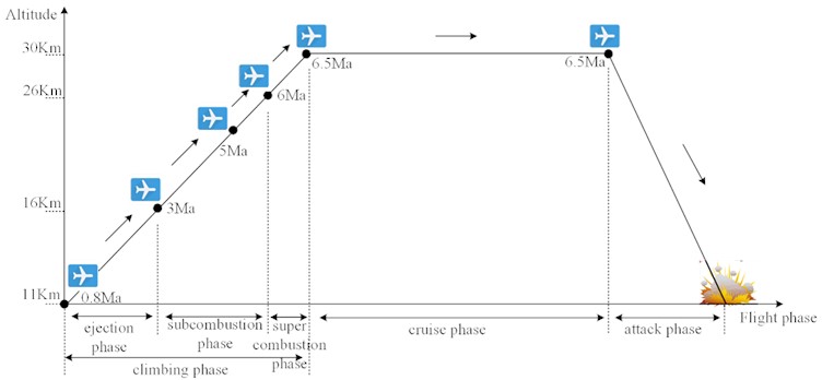
Analyzing the flight trajectory and determining the initial atmospheric conditions is crucial for accurate environmental forecasting. As shown in Fig. 1 [8], the scramjet-propelled vehicle is transported by a large aircraft carrier to the designated location. Subsequently, the solid rocket engine propels the vehicle to achieve Mach 0.8 into the climbing phase, which encompasses the ejection, the sub-combustion, and the super-combustion phases, responsible for rapidly increasing the flight altitude and speed and lasts about 34 seconds. Once the vehicle attains the desired altitude and Mach number (30 km and 6.5), it transitions into the cruise phase. Throughout this period, the vehicle will maintain a consistent altitude and velocity, constituting approximately 90 % of its total range. After reaching the designated airspace, it would proceed to initiate the attack phase with precision and accuracy against the intended target. According to Ref. [9], the external flow field could be categorized as either incompressible or compressible based on its velocity. Furthermore, the compressible flow is considered transonic when the Mach number ranges from 0.6 to 1. The flow field is referred to as supersonic when the Mach number falls between 1 and 3, while it is categorized as high supersonic when the Mach number ranges from 3 to 5. Finally, if the Mach number exceeds 5, the flow field is classified as hypersonic. The flight path of the scramjet-propelled vehicle typically encompasses all the aforementioned compressible conditions. Confirmation of specific environmental prediction parameters is required for different flow conditions. Therefore, it is imperative to analyze the simulation parameters' effect on calculation accuracy to ascertain the optimal simulation configuration. Based on the determined optimal simulation configurations, we could more accurately forecast the aerodynamic conditions of the characteristic position of the scramjet-propelled vehicle during flight, enabling enhanced vehicle optimization and thermal protection design.

Fig. 1The typical flight trajectory of the scramjet-propelled hypersonic vehicle

The NACA0012 airfoil is widely employed for investigating the characteristics of the aerodynamic environment [10]-[14], and the analysis of Refs. [15], [16] reveals a significant correlation between numerical accuracy and the trailing edge shape. NACA0012 has sharp and blunt two trailing edge shapes. For the sharp trailing edge shape, Refs. [17], [18] discusses the external flow field properties of dimpled and square dimpled NACA0012s. The studied Mach numbers are 1.7, 2.2, and 2.7. SST k-omega and Spalart-Allmaras (SA) turbulence models are used. The results show there is a positive correlation between Mach number and aerodynamic condition. Based on different ranges of upper and lower surface temperatures, Ref. [19] extends the previous investigations, and the force coefficients are evaluated. Under the conditions of pitching and plunging NACA0012s, Ref. [20] uses SST k-omega and SA at very low speed to study the thermal effect on force coefficients around NACA0012. The conclusion indicates that the lift coefficient is increased, and the drag coefficient is decreased due to the temperature variation between extrados and intrados of the airfoil. Similar research is investigated by Ref. [21], and a spectral analysis demonstrates that as the surface temperature increases, the force coefficient amplitudes decrease. Based on the 0.3 Mach number and SA model, Ref. [22] discusses water droplets impact characteristics on NACA0012 type turbine, and the calculation results show the matching degree with the experimental results is good, and the numerical approach is acceptable. With an asymmetric heating surface, Ref. [23] selects the k-epsilon turbulence model and Mach number 0.7 to evaluate the NACA0012 anti-icing performance. The research conclusions indicate that the aerodynamic performance could be promoted through the extended heating surface of the suction surface. The impacts of Mach number and ambient temperature on the icing shape and icing growth rate are investigated by Ref. [24], which adopts the SA turbulence model. Regarding the blunt trailing edge, existing literature primarily focuses on noise generation and validation of associated prediction methods, while limited attention has been given to investigating the aerodynamic prediction correlation [25], [26].

In summary, the existing research primarily centers on examining the impact of geometrical alterations on the properties of the external flow field based on a trailing edge shape [27]. There is limited investigation into how the shape of the NACA0012 trailing edge affects the precision of aerodynamic predictions, with only a few studies addressing this aspect [28], [29]. But these studies are all focus on incompressible conditions. During the typical trajectory of hypersonic vehicle shown in Fig. 1, over 90 % of the flight path occurs under hypersonic conditions with a typical Mach number exceeding 5, which is the predominant aerodynamic environment encountered by scramjet-propelled vehicle. However, the maximum Mach number achieved in the aforementioned simulations is below 3, indicating potential deviations from established research conclusions regarding simulation parameter selection for hypersonic conditions. To date, we have not found reliable literature analyzing the influence of trailing edge shape under hypersonic conditions. Meanwhile, the existing literature lacks comprehensive details on the various methodologies employed to establish the NACA0012 model, and the associated CFD simulations commonly incorporate a fixed far field distance and turbulence model. Furthermore, the literature reviewed thus far has paid little attention to the appropriate values of crucial grid parameters such as cell Reynolds number [30] and aspect ratio [31] near the shock, which are characterized by NACA0012. Reliable references addressing the impact of these parameters on numerical accuracy are currently lacking. In summary, there is an insufficient investigation on the selection criteria for these key parameters under hypersonic conditions.

In this study, we select the NACA0012 airfoil as the characterized object to generate computational external flow fields. Our objective is to perform simulations to investigate the influence of trailing edge shape, modeling method, far field distance, and turbulence model on prediction accuracy under hypersonic conditions. By comparing numerical results with wind tunnel data, we establish a correlation between prediction accuracy and simulation parameters and identify an optimal simulation configuration for future reference. This research contributes to the field of environmental prediction for hypersonic flight vehicles. Furthermore, based on the identified optimal simulation configuration mentioned above, we are able to predict environmental conditions along the trajectory of hypersonic vehicle during flight. These predictions provide valuable information for vehicle optimization and thermal protection design.

2. Simulation fundamentals

To look for a suitable simulation scheme for the aerodynamic environment prediction, the appropriate parameter values of the grid strategy and numerical method should be identified through validation tests. $P$ is the local static pressure, and $P_{t}$ is the static pressure of the free stream. $T$ is the local static temperature, and $T_{t}$ is the static temperature of free stream. $U$ is the local velocity, and $U_{t}$ is the velocity of free stream. We adopt the wind tunnel data of $P / P_{t}$ , $T / T_{t}$ and $U / U_{t}$ from Ref. [13] as the reference data, where the location range of $P / P_{t}$ and $T / T_{t}$ is $x / L \in$ [–0.007 0] and the location range of $U / U_{t}$ is $y / L \in$ [0.01 0.1] at $x / L$ = 0.95. The initial values are as follows: Reynolds number ( $R_{e}$ ) is 10e6, the Mach number ( $M_{a}$ ) is 10, $P_{t}$ is 576 Pa, $T_{t}$ is 81.2 K, and the wall temperature of airfoil ( $T_{W}$ ) is 311 K. Ansys ICEM CFD and Ansys fluent are chosen as the meshing tool and the CFD simulation tool, respectively. The calculation process is 16-core parallel, and the precision is double.

2.1. Grid strategy

2.1.1. NACA0012 computational domains

Firstly, we need to choose an appropriate modeling method to design NACA0012 model, which is the basis for establishing computational domain. There exists three NACA0012 modeling methods: NACA4 digital generator, Airfoil tools and definition formula. NACA4 digital generator offers 200 modeling data points and provides the function of the close trailing edge. Therefore, it could be used to design the sharp trailing edge NACA0012 model. Airfoil tools offers 132 modeling data points. The established trailing edge based on this method is not closed and requires a manual connection. So, this method could design the blunt trailing edge. Eq. (1) is the Definition formula, in which the value of $x$ represents the point on the $X$ -axis and the value of y corresponds to the point on the $Y$ -axis. The 200 and 132 $X$ -axis data points offered by NACA4 and Airfoil tools could be substituted into the definition formula to calculate the related Y-axis data points to build the NACA0012 model. In summary, the NACA0012 has two trailing edge shapes, three modeling methods, two data point sources, and different numbers of modeling data points. Therefore, we establish six NACA0012 airfoils, shown in Table 1, to investigate the selection principles of NACA0012 modeling method parameters. Fig. 2 demonstrates the related NACA0012 models, and the airfoil characteristic length ( $L$ ) is 1 m. There exist significant positional differences between different modeling data points:

1

y = \pm 0.5947 [0.2983 x^{1 / 2} - 0.1271 x - 0.3579 x^{2} + 0.2920 x^{3} - 0.1052 x^{4}] .

Table 1The designed six NACA0012s and the corresponding modeling methods

Trailing edge shape	Modeling method
One blunt trailing edge	Airfoil tools (132 points)
Five sharp trailing edges	Naca4 (200 points)
	Definition formula	Adopts 132 points from Airfoil tools
	Definition formula	We double 132 points to 264 points, then substitute them into definition formula
	Definition formula	Adopts 200 points from NACA4
	Definition formula	We double 200 points to 400 points, then substitute them into definition formula

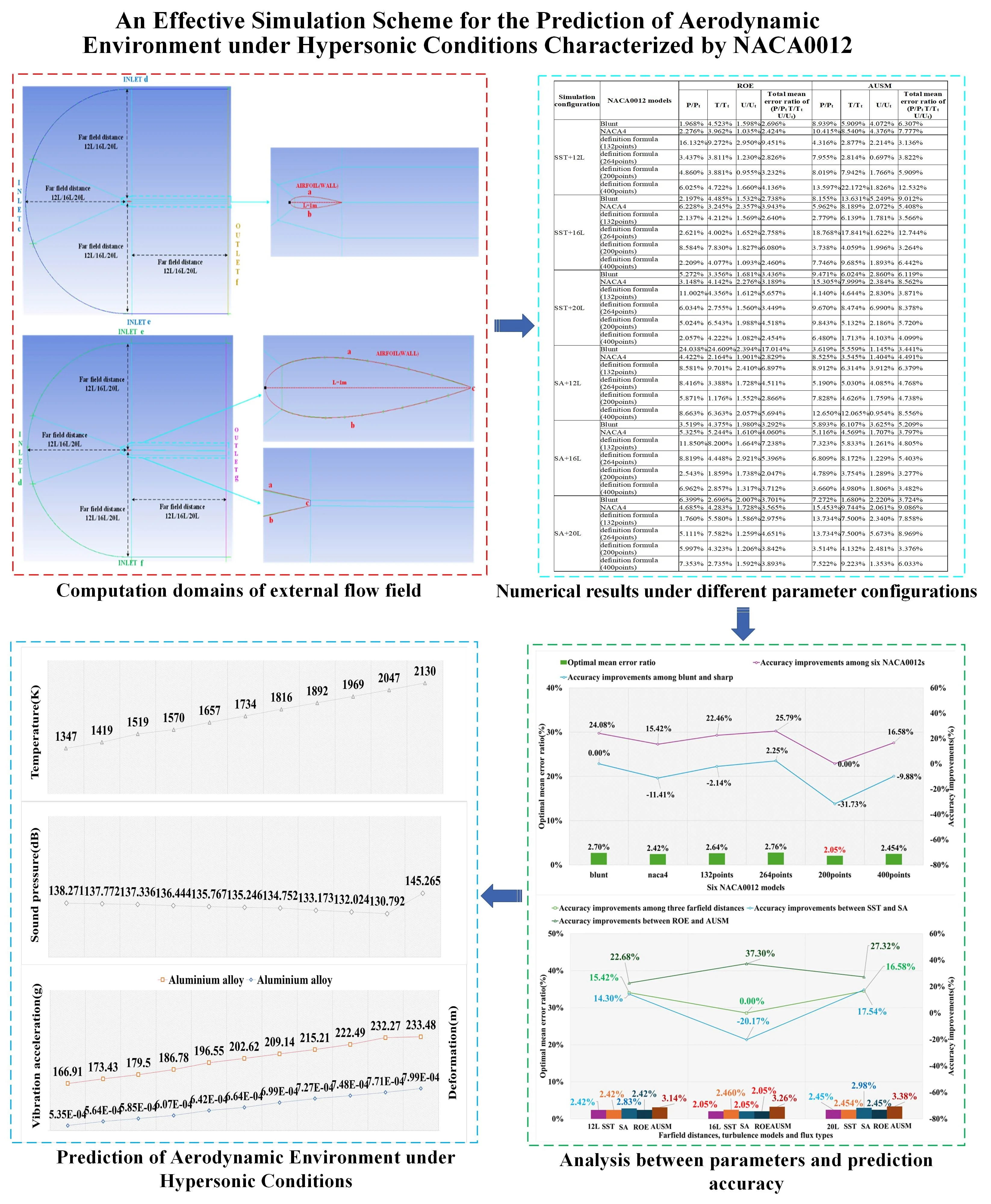
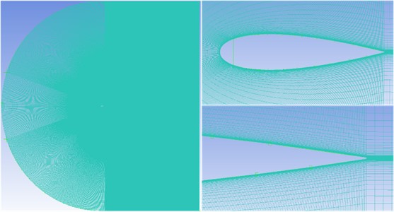
After establishing the NACA0012 models, we need to select the proper far field distance to establish the computational domain of the NACA0012 airfoil to perform numerical simulation. Ansys suggests the far field distance should be 12-20 times $L$ [32]. However, Ansys only provides a suggested range without providing specific values or analyzing the impact of different far field distances on numerical calculation accuracy. By selecting far field distances of 12 $L$ , 16 $L$ , and 20 $L$ and conducting validation tests using wind tunnel data, Ref. [29] examines the correlation between the accuracy of the far field distance in the incompressible external flow field. The findings suggest a discernible relationship between the far field distance and numerical accuracy in the incompressible external flow field. In this study, based on the same research object NACA0012, we still select 12 $L$ /16 $L$ /20 $L$ far field distances to create computational domains. Our investigation focuses on examining the relationship between these distances and numerical accuracy under hypersonic conditions, while also comparing them to incompressible external flow fields [33]. Fig. 3 demonstrates the established two trailing edge types of computational domains, where the black dot is the coordinate origin. The INLET and OUTLET serve as the input and output boundaries, respectively, employing the Pressure far field condition. The WALL boundary, highlighted in red, is characterized by the no-slip, isothermal wall condition. The airfoil surfaces serve as the primary source of the turbulence and the mean vorticity, and the accuracy of numerical predictions for turbulence in wall-bounded flows is heavily influenced by the near-wall meshing. Therefore, finer meshing areas are created by further dividing blocks in close proximity to the airfoil surface. As illustrated in Fig. 3, the cyan lines indicate the grid division. For the sharp trailing edge, the block at the end is folded, whereas it remains in place for the blunt trailing edge.

Fig. 2Six NACA0012 models

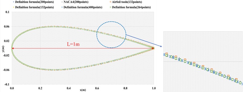
Fig. 3The two types of computational domains

a) Computational domain of the sharp trailing edge and the grid division

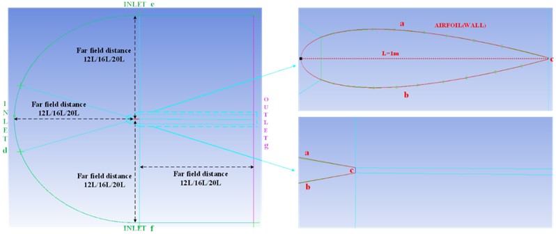
b) Computational domain of the blunt trailing edge and the grid division

2.1.2. Grid parameters

The innermost layer of the near wall is the viscous sublayer, where viscosity has the dominant role in the heat and momentum. The first layer cells of the boundary layer are proposed to exist within the viscous sublayer, with the height value ( $y_{H}$ ) being directly correlated to $y^{+}$ and the calculation process is displayed in Fig. 4. The calculations of $R_{e}$ , $U_{t}$ , air speed ( $C_{a i r}$ ), friction coefficient ( $C_{f}$ ), shear stress ( $τ_{W}$ ), friction velocity ( $μ_{t}$ ), and the distance from the wall to the centroid of the wall adjacent cells ( $y_{p}$ ) are shown from Eqs. (2-8):

2

R_{e} = \frac{ρ U_{t} L}{μ},

3

U_{t} = C_{a i r} \times M_{a},

4

C_{a i r} = 20.05 \sqrt{T_{t}},

5

C_{f} = [2 l o g_{10} (R_{e}) - 0.65]^{- 2.3},

6

τ_{W} = 0.5 \times ρ U^{2} C_{f},

7

u_{τ} = {(\frac{τ_{W}}{ρ})}^{1 / 2},

8

y_{p} = \frac{y^{+} μ}{u_{τ} ρ} .

where $T_{t}$ is 81.2 K and $P_{t}$ is 576 Pa, the flow density ( $ρ$ ) is about 0.0247 kg/m³. $C_{a i r}$ is 180.6 m/s and $M_{a}$ is 10. Hence, $U_{t}$ is 1806m/s. $R_{e}$ is 10e06, $ρ$ , $L$ and $U_{t}$ are substituted into Eq. (2) and flow viscosity ( $μ$ ) is about 4.46082 Pa·s. Then we could solve $y_{p}$ according to Eqs. (5-8). At last, $y_{H}$ is calculated according to Eq. (9):

9

y_{H} = 2 y_{p} .

Fig. 4The calculation process of yH

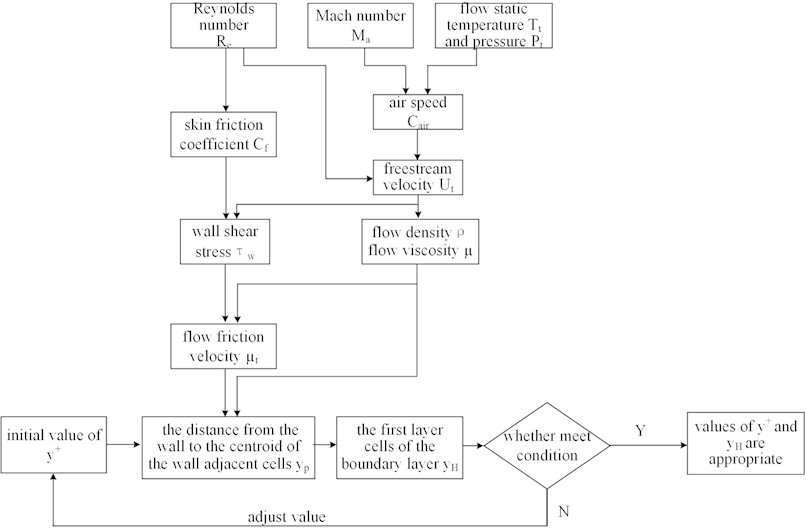
Since the empirical formula ( $C_{f}$ ) is used in the above calculation process [34], $y_{H}$ value is an estimate, and it needs to be tested repeatedly through numerical simulation to ensure that the maximum value of $y^{+}$ at airfoil surface is less than 1 [35]. The initial value of $y^{+}$ is 1, and $y_{H}$ is 4.6e-5 m could be estimated according to the above Equations. However, tests show that the maximum value of $y^{+}$ at the airfoil surface exceeds 1 during simulations, which indicates that the initial value of $y^{+}$ is inappropriate. Through repeated testing, $y^{+}$ is 0.3 and $y_{H}$ is 1.4e-5 m could meet the condition.

Secondly, it is crucial to evaluate the quality of the mesh utilized in a simulation, encompassing an examination of diverse metrics such as aspect ratio and determinant. In particular, meticulous attention must be paid to the aspect ratio since an excessively small value of $y_{H}$ could potentially lead to a large aspect ratio value. This scenario may result in floating-point overflow or calculation divergence, ultimately leading to simulation failure. In this study, we validate the stability of numerical simulations by conducting CFD tests to determine the appropriate aspect ratio and determinant values. At 12 $L$ /16 $L$ /20 $L$ three far field distances, the maximum aspect ratios and the minimum determinants for the sharp and blunt trailing edge shapes are (2100 0.84), (3310 0.881), (4460 0.873) and (2760 0.894), (3680 0.886), (4770 0.827) respectively. These findings ensure the robustness of our numerical simulations.

Fig. 5Mean error ratios of P/Pt, T/Tt, U/Ut at three far field distances under three grid levels (NACA4)

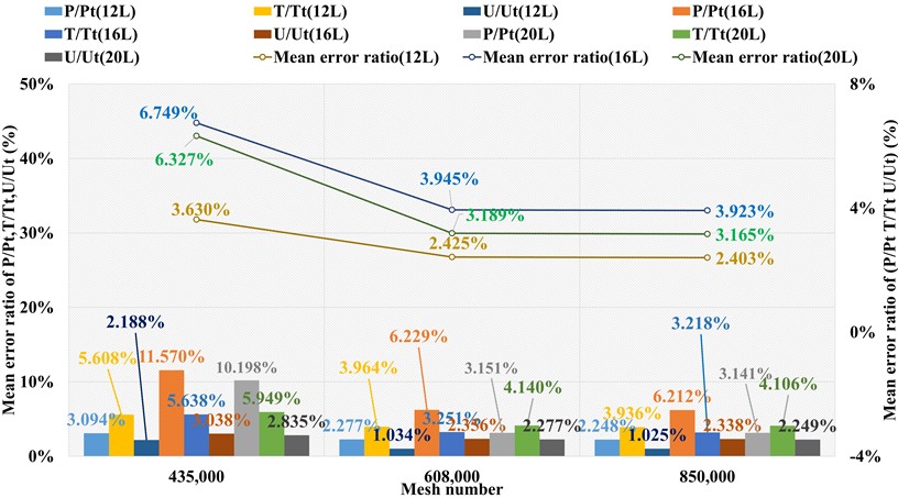
Thirdly, grid independency should be performed to confirm the appropriate total mesh cells number. Three modeling methods are applied to establish three types NACA0012 models: sharp trailing edge (based on NACA4), sharp trailing edge (based on definition formula), and blunt trailing edge (based on Airfoil tools) and we adopt the sharp trailing edge designed by NACA4, combined with the SST k-omega model and ROE flux type as an example. The numerical results of $P / P_{t}$ , $T / T_{t}$ , $U / U_{t}$ at location ranges and related error ratios with wind tunnel data are shown in Fig. 5. At 12 $L$ far field distance, the average error ratios of $P / P_{t}$ , $T / T_{t}$ , and $U / U_{t}$ under three grid levels at all calculating locations are (3.094 % 5.608 % 2.188 %), (2.277 % 3.964 % 1.034 %), and (2.248 % 3.936 % 1.025 %). Hence, the total mean error ratios of ( $P / P_{t}$ $T / T_{t}$ $U / U_{t}$ ) for the three grid levels are 3.630 %, 2.425 %, and 2.403 %. Similarly, the average error ratios for three grid levels under 16L are (11.570 % 5.638 % 3.038 %), (6.229 % 3.251 % 2.356 %), and (6.212 % 3.218 % 2.338 %) and the corresponding total mean error ratios are 6.749 %, 3.945 %, and 3.923 %. The average error ratios under 20 $L$ are (10.198 % 5.949 % 2.835 %), (3.151 % 4.140 % 2.277 %), and (3.141 % 4.106 % 2.249 %) and the corresponding total mean error ratios are 6.327 %, 3.189 %, and 3.165 %. As depicted in Fig. 5, at three far field distance, with the mesh number increases from 608,000 to 850,000, the numerical error ratio hardly changes, and the other two types present similar grid independency performances as shown in Figs. 6 and 7. Therefore, the mesh with 608,000 could meet the requirement of grid independency. The mesh views of the two trailing edge shapes are depicted in Figs. 8-9.

Fig. 6Mean error ratios of P/Pt, T/Tt, U/Ut at three far field distances under three grid levels (Airfoil tools)

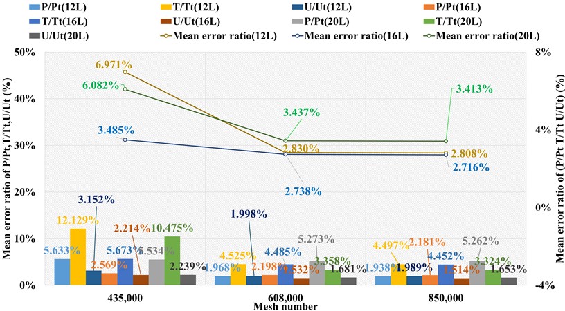
Fig. 7Mean error ratios of P/Pt, T/Tt, U/Ut at three far field distances under three grid levels (Definition formula)

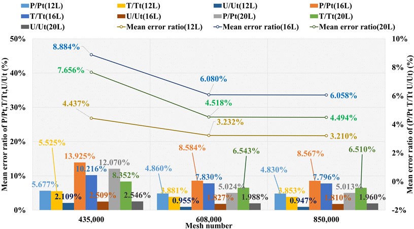
Fig. 8The mesh views of the sharp trailing edge

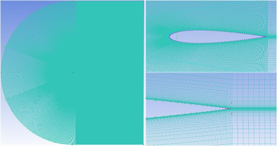
Fig. 9The mesh views of the blunt trailing edge

2.2. Numerical method

2.2.1. Turbulence model

When working with transonic fluids, it is necessary to manage compression and heat transfer. This necessitates solving control equations such as mass continuity, momentum (the NS equation), and energy. Since turbulent flow exists, additional transport equations must be solved. Turbulence is defined as unsteady random motion in fluids with medium to high Reynolds numbers, as described by the NS equation. However, direct numerical simulation (DNS) calculations can be time-consuming, necessitating the averaging of the NS equation to reduce turbulence components. The Reynolds Averaged Navier-Stokes (RANS) model is widely used to average the turbulence fluctuation time term. This method employs turbulent viscosity to calculate Reynolds stress and solve the RANS equations. The k-epsilon, SST k-omega, and Spalart-Allmaras (SA) turbulence models are widely accepted and relatively accurate for most numerical simulation applications [36]. However, the k-epsilon model exhibits limited sensitivity to adverse pressure gradients and boundary layer separation, resulting in delayed predictions and separation. Consequently, it is unsuitable for investigating the aerodynamic external flow field in this paper. The k-omega model demonstrates superior performance over the k-epsilon model in predicting adverse pressure gradients and boundary layer flow, showcasing its enhanced capabilities. Furthermore, the SST k-omega model effectively addresses the sensitivity issue of the original k-omega model to freestream conditions, thereby enhancing its applicability [37]. Moreover, the Spalart-Allmaras (SA) turbulence model is specifically tailored for aerospace applications involving wall-bounded flows and exhibits exceptional predictive capabilities for adverse pressure gradient boundary layers [38]. In conclusion, we employ SA and SST k-omega models.

Regarding the INLET boundary, when utilizing the SST k-omega, we employ the intensity and viscosity ratio turbulence method with values of 1 % and 1. In case of adopting the SA model, the turbulent viscosity ratio method is chosen and set its value to 1. The same actions are done for the OUTLET boundary. Furthermore, careful consideration should be given to selecting an appropriate upwind order for modifying turbulent viscosity in relation to the SA model. According to Ref. [30], there exists a situation where the performance of the first order is better than that of the second order. So, we execute a numerical comparison between these two upwind schemes. We still take the sharp trailing edge designed by NACA4, combined with ROE flux type as an example to carry out the analysis. The numerical results of $P / P_{t}$ , $T / T_{t}$ , and $U / U_{t}$ at location ranges and related error ratios with wind tunnel data are shown in Tables 2-4. For the first order, under three far field distances, the mean error ratios of ( $P / P_{t}$ , $T / T_{t}$ and $U / U_{t}$ ) at all calculating locations are (9.18 % 4.96 % 3.02 %), (9.38 % 7.71 % 2.06 %), and (7.42 % 7.11 % 2.72 %). The corresponding total mean error ratios of ( $P / P_{t}$ $T / T_{t}$ $U / U_{t}$ ) are 5.72 %, 6.38 %, and 5.75 %. Similarly, for the second order, the mean error ratios under three far field distances are (4.42 % 2.16 % 1.90 %), (5.33 % 5.24 % 1.61 %), and (4.69 % 4.28 % 1.73 %), and the total mean error ratios are 2.83 %, 4.06 %, and 3.57 %. Hence, the second order upwind is chosen.

Table 2Numerical results comparison of P/Pt between the first-order upwind and second–order upwind of the modified turbulent viscosity

Type of upwind order	$x$ / $L$ locations (m) and $P$ / $P_{t}$ wind tunnel data ( $P$ / $P_{t}$ numerical results and error ratios)
	–0.007		–0.006	–0.005	–0.004	–0.003	–0.002	–0.001	0
	103.63		114.55	117.87	119.40	121.74	122.10	123.39	123.83
First-order	12 $L$	81.68	106.49	114.80	110.43	110.71	112.04	112.79	112.42
	12 $L$	21.19 %	7.04 %	2.60 %	7.51 %	9.06 %	8.24 %	8.59 %	9.22 %
	16 $L$	63.99	101.22	118.76	117.55	120.54	125.16	134.83	136.33
	16 $L$	38.25 %	11.64 %	0.76 %	1.55 %	0.99 %	2.51 %	9.27 %	10.10 %
	20 $L$	107.09	106.96	105.16	105.66	106.74	110.22	118.13	122.88
	20 $L$	3.34 %	6.63 %	10.79 %	11.5 %	12.32 %	9.73 %	4.27 %	0.77 %
Second-order	12 $L$	93.15	112.16	117.71	119.13	122.20	125.88	134.72	136.43
	12 $L$	10.11 %	2.09 %	0.14 %	0.23 %	0.38 %	3.10 %	9.18 %	10.17 %
	16 $L$	106.92	112.50	115.21	115.48	115.45	115.19	113.54	107.39
	16 $L$	3.18 %	1.79 %	2.26 %	3.28 %	5.17 %	5.66 %	7.99 %	13.28 %
	20 $L$	102.75	106.52	113.59	117.72	122.04	126.47	136.72	136.17
	20 $L$	0.85 %	7.01 %	3.63 %	1.41 %	0.25 %	3.58 %	10.8 %	9.96 %

Table 3Numerical results comparison of T/Tt between the first-order upwind and second-order upwind of the Modified turbulent viscosity

Type of upwind order	$x$ / $L$ locations (m) and $T$ / $T_{t}$ wind tunnel data ( $T$ / $T_{t}$ numerical results and error ratios)
	–0.007		–0.006	–0.005	–0.004	–0.003	–0.002	–0.001	0
	18.15		20.19	20.28	20.43	20.52	20.66	21.04	21.33
First-order	12 $L$	15.34	18.71	20.36	20.78	20.86	20.79	20.39	19.33
	12 $L$	15.50 %	7.31 %	0.38 %	1.70 %	1.68 %	0.65 %	3.11 %	9.35 %
	16 $L$	12.08	17.15	20.02	20.13	20.30	20.53	20.44	20.07
	16 $L$	33.47 %	15.03 %	1.26 %	1.49 %	1.07 %	0.62 %	2.83 %	5.91 %
	20 $L$	19.59	19.92	19.86	19.62	19.58	20.02	20.44	14.71
	20 $L$	7.96 %	1.32 %	2.09 %	3.96 %	4.57 %	3.09 %	2.87 %	31.04 %
Second-order	12 $L$	17.55	19.13	20.06	20.17	20.30	20.55	20.64	20.71
	12 $L$	3.28 %	5.24 %	1.08 %	1.25 %	1.08 %	0.52 %	1.89 %	2.92 %
	16 $L$	19.57	20.03	20.26	20.33	20.31	20.47	20.10	15.72
	16 $L$	7.82 %	0.79 %	0.07 %	0.51 %	1.03 %	0.92 %	4.46 %	26.3 %
	20 $L$	20.47	20.33	20.20	20.06	20.08	20.11	20.29	19.16
	20 $L$	12.79 %	0.68 %	0.39 %	1.79 %	2.17 %	2.68 %	3.58 %	10.18 %

Table 4Numerical results comparison of U/Ut between the first-order upwind and second-order upwind of the modified turbulent viscosity

Type of upwind order		$y$ / $L$ locations (m) at $x$ / $L =$ 0.95 m ( $U$ / $U_{t}$ numerical results and error ratios)
		0.01	0.02	0.03	0.04	0.05	0.06	0.07	0.08	0.09	0.1
		0.6907	0.8199	0.8556	0.8667	0.8705	0.8711	0.8740	0.8746	0.8771	0.8801
First- order	12 $L$	0.6315	0.8444	0.8823	0.8837	0.8858	0.8899	0.8920	0.8963	0.9020	0.8997
	12 $L$	8.56 %	2.98 %	3.13 %	1.97 %	1.75 %	2.16 %	2.06 %	2.49 %	2.84 %	2.22 %
	16 $L$	0.6392	0.8383	0.8668	0.8606	0.8737	0.8797	0.8883	0.8892	0.8943	0.8998
	16 $L$	7.46 %	2.24 %	1.31 %	0.71 %	0.36 %	0.98 %	1.63 %	1.67 %	1.96 %	2.23 %
	20 $L$	0.6487	0.8456	0.8862	0.8895	0.8865	0.8852	0.8904	0.8933	0.8971	0.8983
	20 $L$	6.08 %	3.13 %	3.57 %	2.64 %	1.84 %	1.61 %	1.88 %	2.15 %	2.29 %	2.06 %
Second- order	12 $L$	0.6405	0.8374	0.8733	0.8777	0.8795	0.8807	0.8820	0.8843	0.8870	0.8887
	12 $L$	7.26 %	2.13 %	2.07 %	1.27 %	1.02 %	1.10 %	0.92 %	1.12 %	1.13 %	0.97 %
	16 $L$	0.6339	0.8357	0.8624	0.8666	0.8707	0.8756	0.8801	0.8851	0.8893	0.8918
	16 $L$	8.23 %	1.93 %	0.79 %	0.01 %	0.01 %	0.51 %	0.69 %	1.20 %	1.39 %	1.32 %
	20 $L$	0.6547	0.8416	0.8802	0.8815	0.8795	0.8788	0.8794	0.8816	0.8841	0.8863
	20 $L$	5.21 %	2.64 %	2.87 %	1.71 %	1.03 %	0.88 %	0.62 %	0.81 %	0.81 %	0.70 %

2.2.2. Flux type and spatial discretization

An appropriate scheme is needed to evaluate the flux component. According to Ref. [39], the cylinder is taken as a research object to investigate the simulation performance of different flux types, and the conclusions demonstrate that the results of the ROE and AUSM are closer to the reference data. Therefore, we adopt these two types to study the capability of the simulation accuracy of aerodynamic prediction characterized by NACA0012 under hypersonic conditions. For the flow discretization, the second order upwind is selected. A suitable gradient calculation scheme is also needed, based on which the cell face scalar values could be constructed. The calculation of related diffusion terms and velocity derivatives can be done. There are three types of schemes (node-based/cell-based/least cell-based). Out of these three, the least cell-based scheme is advantageous because it provides comparable accuracy to the node-based scheme, has fewer computing resources, and avoids spurious oscillations. Hence, the least cell-based with the standard gradient limiter is applied. In addition, when the Mach number is bigger than 5, the density-based solver is employed. Since the Mach number of validation tests is 10, it should be considered whether there exists real gas effect. The air critical pressure ( $P_{c}$ ) is 3.77 MPa, and if the ratio of $P$ and $P_{c}$ is much less than 1, then we could select the ideal gas. During the numerical simulation process, the value of $P$ increases from the initial 576 Pa to the maximum 73728 Pa. The maximum ratio of $P$ and $P_{c}$ is about 0.019, which satisfies the condition mentioned above. Hence, flow density ( $ρ$ ) selects the ideal gas.

3. Numerical results and discussion

3.1. Numerical results

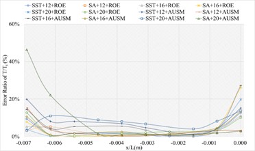
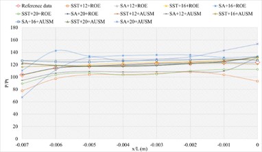
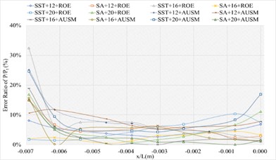
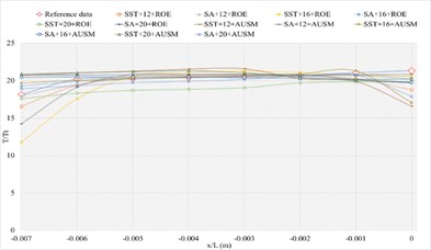
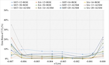
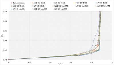
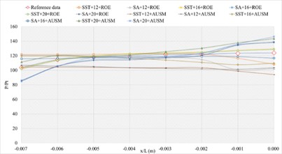
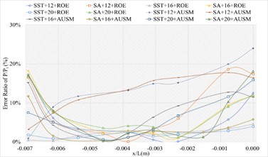
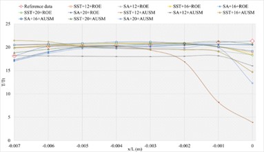
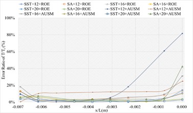
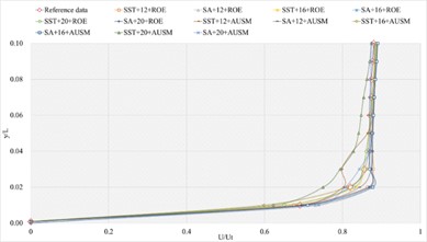
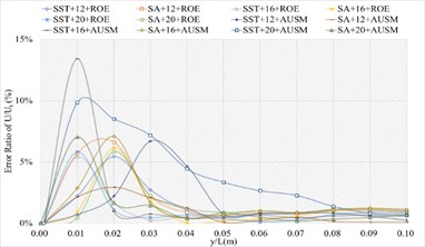
Based on the description in Grid strategy and Numerical Method, we apply six NACA0012 models, three far field distances, two turbulence models and two flux types to construct the simulation configurations and a total of seventy-two sets of numerical calculations are carried out. Tables 5-22 demonstrate the numerical results of $P / P_{t}$ , $T / T_{t}$ , $U / U_{t}$ at sampling locations and Figs. 10-15 demonstrate the corresponding numerical error ratio distributions of $P / P_{t}$ , $T / T_{t}$ , $U / U_{t}$ compared with the wind tunnel data. The bold black values in the tables below $x$ / $L$ sampling positions represent the corresponding wind tunnel test data, and the red dashed diamond shapes in the figures indicate wind tunnel data at those positions. Table 23 demonstrates the mean error ratios of $P / P_{t}$ , $T / T_{t}$ , $U / U_{t}$ for six NACA0012 models under different simulation configurations. Through the error ratio comparison, the optimal mean error ratio of ( $P / P_{t}$ $T / T_{t}$ $U / U_{t}$ ) of 2.05 % could be achieved based on the configuration of sharp trailing edge (definition formula) + 16 $L$ far field distance + SA turbulence model + ROE flux type.

Table 5Numerical results of P/Pt of blunt trailing edge adopting two turbulence models, three far field distances and two flux types

NACA0012 models		$x$ / $L$ (m) and $P$ / $P_{t}$ wind tunnel data ( $P$ / $P_{t}$ numerical data)
		–0.007	–0.006	–0.005	–0.004	–0.003	–0.002	–0.001	0
		103.6285	114.5508	117.8656	119.3983	121.7447	122.1036	123.3942	123.8330
SST+12 $L$	ROE	103.1758	114.2245	119.3853	122.5377	123.7579	124.7891	127.2207	128.9688
SST+12 $L$	AUSM	115.2700	114.4670	115.0006	114.7569	113.8172	111.8231	102.0335	97.0301
SA+12 $L$	ROE	6.0925	35.2682	107.9680	118.2251	118.7486	121.5961	129.3444	138.5572
SA+12 $L$	AUSM	113.6156	114.3060	113.3640	113.4916	114.8708	118.5805	122.1218	124.7841
SST+16 $L$	ROE	101.3087	113.2991	119.0844	122.3194	123.5652	124.6285	127.1412	128.9871
SST+16 $L$	AUSM	126.2989	125.2276	124.6631	126.3320	127.7393	129.1166	123.0015	109.6105
SA+16 $L$	ROE	112.1930	112.6418	113.9845	114.8477	115.8725	120.3363	125.7635	127.4569
SA+16 $L$	AUSM	115.5999	116.4176	117.9377	122.8046	126.0157	129.6497	135.4119	138.2230
SST+20 $L$	ROE	108.5238	119.5044	122.4766	125.7646	127.0867	128.2546	131.3245	133.7835
SST+20 $L$	AUSM	85.9375	103.1402	111.8435	111.6520	111.9114	112.0232	111.3510	110.1554
SA+20 $L$	ROE	88.2687	113.0102	122.2196	123.6521	126.3275	128.9982	134.4160	135.5053
SA+20 $L$	AUSM	108.2922	118.8877	118.7423	122.1060	125.9117	129.5463	140.4347	152.9953

Table 6Numerical results of T/Tt of blunt trailing edge shape adopting two turbulence models, three far field distances and two flux types

NACA0012 models		$x$ / $L$ (m) and $T$ / $T_{t}$ wind tunnel data ( $T$ / $T_{t}$ numerical data)
		–0.007	–0.006	–0.005	–0.004	–0.003	–0.002	–0.001	0
		18.152	20.190	20.284	20.427	20.521	20.664	21.043	21.327
SST+12 $L$	ROE	19.918	20.418	20.675	20.792	20.765	20.680	20.151	17.892
SST+12 $L$	AUSM	20.097	20.334	20.580	20.726	20.290	19.677	18.936	17.701
SA+12 $L$	ROE	1.996	7.765	18.344	18.839	18.886	18.838	18.760	21.042
SA+12 $L$	AUSM	18.489	18.647	18.768	18.914	19.123	19.572	19.940	20.739
SST+16 $L$	ROE	19.825	20.387	20.678	20.805	20.785	20.708	20.191	17.840
SST+16 $L$	AUSM	20.592	20.758	20.866	20.959	20.879	20.700	18.750	5.439
SA+16 $L$	ROE	20.483	20.664	20.806	20.898	20.907	20.604	19.867	19.799
SA+16 $L$	AUSM	21.109	21.046	20.979	21.037	21.168	21.327	21.626	18.600
SST+20 $L$	ROE	18.909	20.412	20.572	20.688	20.685	20.628	20.178	18.384
SST+20 $L$	AUSM	17.365	19.335	19.951	20.074	20.074	20.443	20.074	15.271
SA+20 $L$	ROE	16.506	19.037	20.212	20.459	20.567	20.657	20.795	20.293
SA+20 $L$	AUSM	18.681	19.851	20.331	20.683	20.925	21.156	20.720	21.642

Table 7Numerical results of U/Ut of blunt trailing edge adopting two turbulence models, three far field distances and two flux types

NACA0012 models		$y$ / $L$ (m) at $x$ / $L$ = 0.95 m and $U$ / $U_{t}$ wind tunnel data ( $U$ / $U_{t}$ numerical data)
		0.01	0.02	0.03	0.04	0.05	0.06	0.07	0.08	0.09	0.1
		0.6907	0.8199	0.8556	0.8667	0.8705	0.8711	0.8740	0.8746	0.8771	0.8801
SST+12 $L$	ROE	0.5939	0.8335	0.8538	0.8620	0.8680	0.8733	0.8774	0.8818	0.8855	0.8876
SST+12 $L$	AUSM	0.5529	0.7516	0.7981	0.8395	0.8628	0.8714	0.8720	0.8719	0.8731	0.8742
SA+12 $L$	ROE	0.6364	0.8604	0.8746	0.8881	0.8845	0.8826	0.8825	0.8832	0.8849	0.8861
SA+12 $L$	AUSM	0.6481	0.8350	0.8642	0.8657	0.8711	0.8769	0.8792	0.8796	0.8802	0.8807
SST+16 $L$	ROE	0.6323	0.8421	0.8568	0.8639	0.8695	0.8744	0.8782	0.8823	0.8858	0.8878
SST+16 $L$	AUSM	0.5359	0.7300	0.7756	0.8271	0.8548	0.8636	0.8694	0.8773	0.8841	0.8879
SA+16 $L$	ROE	0.6659	0.8723	0.8732	0.8730	0.8763	0.8807	0.8840	0.8871	0.8897	0.8912
SA+16 $L$	AUSM	0.6365	0.7868	0.7936	0.8110	0.8432	0.8701	0.8841	0.8928	0.8965	0.8976
SST+20 $L$	ROE	0.6212	0.8438	0.8581	0.8646	0.8696	0.8740	0.8775	0.8814	0.8849	0.8871
SST+20 $L$	AUSM	0.5947	0.8718	0.8651	0.8665	0.8782	0.8853	0.8871	0.8863	0.8866	0.8873
SA+20 $L$	ROE	0.6567	0.8747	0.8762	0.8766	0.8772	0.8783	0.8798	0.8823	0.8853	0.8873
SA+20 $L$	AUSM	0.6249	0.8669	0.8788	0.8777	0.8738	0.8741	0.8762	0.8800	0.8836	0.8858

3.1.1. Airfoil tools

The corresponding numerical results and distributions of $P / P_{t}$ , $T / T_{t}$ and $U / U_{t}$ are shown in Tables 5-7 and Fig. 10. Table 23 provides the mean error ratios under different simulation configurations. From the aspect of far field distance, the minimum values are 2.696 %, 2.738 %, and 3.436 % in order. From the aspect of turbulence model, the most favorable outcome for SST is 2.696 %, while that of SA is 3.292 %. For the two flux types, the finest value of ROE is 2.696 % and that of AUSM is 3.441 %. In conclusion, the SST+12 $L$ configuration, combined with ROE has achieved the minimum total mean error ratio. Compared with other simulation configurations, the corresponding accuracy improvements are 57.249 %, 84.153 %, 21.642 %, 1.532 %, 70.082 %, 18.089 %, 48.237 %, 21.543 %, 55.935 %, 27.146 %, and 27.602 %, respectively.

Fig. 10The numerical result and error ratio distributions of P/Pt, T/Tt and U/Ut of blunt trailing edge

a) Numerical result distribution of $P$ / $P_{t}$ of the blunt trailing edge

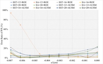
b) Error ratio distribution of $P$ / $P_{t}$ of the blunt trailing edge

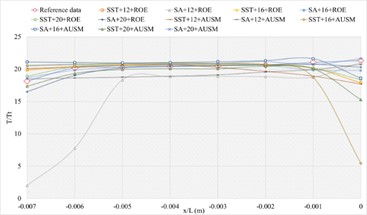
c) Numerical result distribution of $T$ / $T_{t}$ of the blunt trailing edge

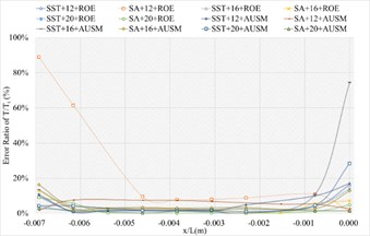
d) Error ratio distribution of $T$ / $T_{t}$ of the blunt trailing edge

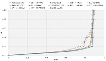
e) Numerical result distribution of $U$ / $U_{t}$ of the blunt trailing edge

f) Error ratio distribution of $U$ / $U_{t}$ of the blunt trailing edge

3.1.2. NACA4

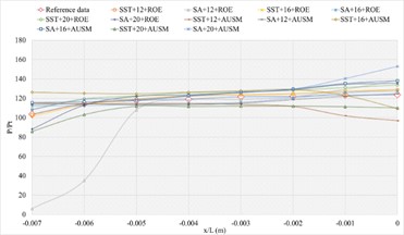
The corresponding numerical results and distributions of $P / P_{t}$ , $T / T_{t}$ and $U / U_{t}$ are shown in Tables 8-10 and Fig. 11. Table 23 provides the mean error ratios under different simulation configurations. From the aspect of far field distance, the minimum values are 2.420 %, 3.797 %, and 3.189 % in order. From the aspect of turbulence model, the most favorable outcome for SST is 2.420 %, while that of SA is 2.829 %. For the two flux types, the finest value of ROE is 2.420 % and that of AUSM is 3.797 %.

Table 8Numerical results of P/Pt of sharp trailing edge based on NACA4 adopting two turbulence models, three far field distances and two flux types

NACA0012 models		$x$ / $L$ (m) and $P$ / $P_{t}$ wind tunnel data ( $P$ / $P_{t}$ numerical data)
		–0.007	–0.006	–0.005	–0.004	–0.003	–0.002	–0.001	0
		103.6285	114.5508	117.8656	119.3983	121.7447	122.1036	123.3942	123.8330
SST+12 $L$	ROE	102.6623	113.7859	119.5540	122.7781	124.0214	125.0571	127.6113	129.5765
SST+12 $L$	AUSM	125.0601	122.6266	123.4892	130.3869	133.7133	136.7315	138.2960	133.3994
SA+12 $L$	ROE	93.1517	112.1581	117.7100	119.1311	122.1984	125.8803	134.7221	136.4293
SA+12 $L$	AUSM	120.0194	113.7502	110.6636	109.2987	109.0662	109.8360	111.0621	115.5866
SST+16 $L$	ROE	90.3901	114.5756	124.3798	125.3509	127.3098	128.9722	132.1900	135.2095
SST+16 $L$	AUSM	123.6560	124.3612	124.9024	124.9201	124.3482	122.1458	119.9241	118.5962
SA+16 $L$	ROE	106.9225	112.5033	115.2072	115.4793	115.4510	115.1886	113.5401	107.3866
SA+16 $L$	AUSM	118.0516	119.6460	120.2279	120.3639	120.1021	119.3604	115.6705	111.5844
SST+20 $L$	ROE	91.5191	108.2494	117.8706	120.9798	122.3012	123.3865	125.8781	127.7352
SST+20 $L$	AUSM	98.4080	99.3577	98.2276	97.5850	97.8597	100.8383	103.7027	103.7561
SA+20 $L$	ROE	102.7478	106.5220	113.5859	117.7168	122.0448	126.4707	136.7221	136.1655
SA+20 $L$	AUSM	37.4234	73.3389	117.5831	118.8793	121.1027	123.9634	132.9692	140.2752

Table 9Numerical results of T/Tt of sharp trailing edge based on NACA4 adopting two turbulence models, three far field distances and two flux types

NACA0012 models		$x$ / $L$ (m) and $T$ / $T_{t}$ wind tunnel data ( $T$ / $T_{t}$ numerical data)
		–0.007	–0.006	–0.005	–0.004	–0.003	–0.002	–0.001	0
		18.152	20.190	20.284	20.427	20.521	20.664	21.043	21.327
SST+12 $L$	ROE	19.860	20.361	20.640	20.773	20.761	20.693	20.219	18.605
SST+12 $L$	AUSM	21.769	21.834	21.924	21.832	21.495	20.869	20.137	18.077
SA+12 $L$	ROE	17.555	19.131	20.061	20.174	20.297	20.552	20.642	20.707
SA+12 $L$	AUSM	20.927	20.926	20.499	20.374	20.430	20.417	20.365	20.634
SST+16 $L$	ROE	17.182	19.264	20.271	20.609	20.704	20.696	20.454	18.930
SST+16 $L$	AUSM	20.769	21.064	21.367	21.568	21.237	20.772	20.092	15.503
SA+16 $L$	ROE	19.570	20.031	20.265	20.325	20.309	20.469	20.101	15.717
SA+16 $L$	AUSM	20.084	20.383	20.633	20.941	20.775	20.338	20.090	18.476
SST+20 $L$	ROE	18.834	20.122	20.647	20.833	20.832	20.610	20.262	17.108
SST+20 $L$	AUSM	17.580	17.965	18.472	18.797	19.136	19.811	19.313	18.382
SA+20 $L$	ROE	20.471	20.327	20.202	20.064	20.075	20.107	20.287	19.159
SA+20 $L$	AUSM	9.741	15.713	20.595	20.631	20.719	20.863	20.630	20.683

Table 10Numerical results of U/Ut of sharp trailing edge based on NACA4 adopting two turbulence models, three far field distances and two flux types

NACA0012 models		$y$ / $L$ (m) at $x$ / $L$ = 0.95 m and $U$ / $U_{t}$ wind tunnel data ( $U$ / $U_{t}$ numerical data)
		0.01	0.02	0.03	0.04	0.05	0.06	0.07	0.08	0.09	0.1
		0.6907	0.8199	0.8556	0.8667	0.8705	0.8711	0.8740	0.8746	0.8771	0.8801
SST+12 $L$	ROE	0.6547	0.8416	0.8802	0.8815	0.8795	0.8788	0.8794	0.8816	0.8841	0.8863
SST+12 $L$	AUSM	0.6162	0.7966	0.8333	0.8513	0.8659	0.8776	0.8842	0.8870	0.8870	0.8873
SA+12 $L$	ROE	0.5989	0.7913	0.8351	0.8549	0.8648	0.8712	0.8757	0.8803	0.8841	0.8864
SA+12 $L$	AUSM	0.6515	0.8304	0.8604	0.8849	0.8960	0.8948	0.8907	0.8876	0.8871	0.8872
SST+16 $L$	ROE	0.6405	0.8374	0.8733	0.8777	0.8795	0.8807	0.8820	0.8843	0.8870	0.8887
SST+16 $L$	AUSM	0.5989	0.8126	0.8572	0.8667	0.8717	0.8770	0.8818	0.8871	0.8913	0.8938
SA+16 $L$	ROE	0.5957	0.7883	0.8337	0.8542	0.8642	0.8708	0.8755	0.8805	0.8845	0.8869
SA+16 $L$	AUSM	0.6457	0.8428	0.8642	0.8679	0.8722	0.8775	0.8822	0.8875	0.8917	0.8942
SST+20 $L$	ROE	0.6070	0.7921	0.8348	0.8547	0.8650	0.8718	0.8766	0.8813	0.8848	0.8868
SST+20 $L$	AUSM	0.5712	0.7690	0.7879	0.8170	0.8482	0.8685	0.8784	0.8839	0.8872	0.8889
SA+20 $L$	ROE	0.6339	0.8357	0.8624	0.8666	0.8707	0.8756	0.8801	0.8851	0.8893	0.8918
SA+20 $L$	AUSM	0.6564	0.8019	0.8492	0.8747	0.8793	0.8809	0.8820	0.8828	0.8836	0.8842

In conclusion, the SST+12 $L$ configuration, combined with ROE has achieved the minimum mean error ratio. Compared with other simulation configurations, the corresponding accuracy improvements are 68.882 %, 14.453 %, 46.120 %, 38.628 %, 55.249 %, 40.390 %, 36.269 %, 24.114 %, 71.737 %, 32.125 %, and 73.366 %, respectively.

Fig. 11The numerical result and error ratio distributions of P/Pt, T/Tt and U/Ut of sharp trailing edge based on NACA4

a) Numerical result distribution of $P / P_{t}$ of the sharp trailing edge based on NACA4

b) Error ratio distribution of $P / P_{t}$ of the sharp trailing edge based on NACA4

c) Numerical result distribution of $T / T_{t}$ of the sharp trailing edge based on NACA4

d) Error ratio distribution of $T / T_{t}$ of the sharp trailing edge based on NACA4

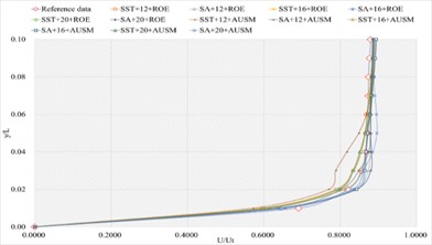
e) Numerical result distribution of $U / U_{t}$ of the sharp trailing edge based on NACA4

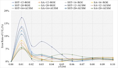
f) Error ratio distribution of $U / U_{t}$ of the sharp trailing edge based on NACA4

3.1.3. Definition formula adopting 132 points

The corresponding numerical results and distributions of $P / P_{t}$ , $T / T_{t}$ and $U / U_{t}$ are shown in Tables 11-13 and Fig.12. Table 23 provides the mean error ratios under different simulation configurations. From the aspect of far field distance, the minimum values are 3.136 %, 2.640 %, and 2.975 % in order. From the aspect of turbulence model, the most favorable outcome for SST is 2.640 %, while that of SA is 2.975 %. For the two flux types, the finest value of ROE is 2.640 % and that of AUSM is 3.136 %. In conclusion, the SST+16 $L$ configuration, combined with ROE has achieved the minimum mean error ratio. Compared with other simulation configurations, the corresponding accuracy improvements are72.073 %, 15.821 %, 61.731 %, 58.624 %, 25.987 %, 63.533 %, 45.070 %, 53.338 %, 31.817 %, 11.290 %, and 66.411 %, respectively.

Table 11Numerical results of P/Pt of sharp trailing edge based on definition formula (132 points) adopting two turbulence models, three far field distances and two flux types

NACA0012 models		$x$ / $L$ (m) and $P$ / $P_{t}$ wind tunnel data ( $P$ / $P_{t}$ numerical data)
		–0.007	–0.006	–0.005	–0.004	–0.003	–0.002	–0.001	0
		103.6285	114.5508	117.8656	119.3983	121.7447	122.1036	123.3942	123.8330
SST+12 $L$	ROE	77.9720	97.5837	103.9596	104.2068	105.7531	108.2004	103.7853	93.4325
SST+12 $L$	AUSM	122.9772	118.5715	117.4966	120.4748	122.3124	123.9481	126.0108	132.5421
SA+12 $L$	ROE	126.8481	127.4266	128.1201	128.9839	128.9838	128.9172	128.3850	127.1818
SA+12 $L$	AUSM	94.8265	106.4431	109.2256	108.2244	108.7156	108.9666	109.8323	131.9843
SST+16 $L$	ROE	102.8513	114.0935	119.5973	122.7339	123.9256	124.9008	127.3781	129.2507
SST+16 $L$	AUSM	116.3570	118.2875	117.5792	117.6293	119.3575	122.0409	122.4785	121.0955
SA+16 $L$	ROE	110.5474	142.6264	133.8498	134.7360	135.7823	135.8110	131.7480	133.3460
SA+16 $L$	AUSM	126.5742	124.6259	124.2431	126.2068	126.8411	127.7232	129.5196	127.2727
SST+20 $L$	ROE	89.3645	103.6540	106.7764	103.4379	104.8373	109.8622	112.3890	112.5213
SST+20 $L$	AUSM	121.9440	118.9971	117.6949	118.6125	119.4331	121.7822	125.1382	132.7346
SA+20 $L$	ROE	103.6814	114.6149	117.3158	116.9946	118.5445	122.0046	125.1439	132.9575
SA+20 $L$	AUSM	67.4088	111.4342	132.0675	125.9648	128.9382	132.7707	143.0583	153.6435

Table 12Numerical results of T/Tt of sharp trailing edge based on definition formula (132 points) adopting two turbulence models, three far field distances and two flux types

NACA0012 models		$x$ / $L$ (m) and $T$ / $T_{t}$ wind tunnel data ( $T$ / $T_{t}$ numerical data)
		–0.007	–0.006	–0.005	–0.004	–0.003	–0.002	–0.001	0
		18.152	20.190	20.284	20.427	20.521	20.664	21.043	21.327
SST+12 $L$	ROE	15.133	16.859	18.502	19.281	20.050	20.660	19.174	18.030
SST+12 $L$	AUSM	19.944	20.075	20.212	20.495	20.646	20.841	21.900	19.971
SA+12 $L$	ROE	20.816	20.841	20.869	20.909	20.932	20.995	20.806	10.720
SA+12 $L$	AUSM	17.497	18.624	19.302	19.408	19.484	19.593	19.665	18.654
SST+16 $L$	ROE	19.873	20.384	20.656	20.781	20.761	20.683	20.173	18.277
SST+16 $L$	AUSM	18.708	19.203	19.657	19.851	20.044	20.498	20.571	14.955
SA+16 $L$	ROE	16.122	20.522	22.666	23.641	23.466	20.439	19.578	20.710
SA+16 $L$	AUSM	21.319	21.230	21.041	20.932	20.794	20.698	21.178	17.974
SST+20 $L$	ROE	17.271	19.272	20.199	20.584	20.672	20.630	19.591	17.817
SST+20 $L$	AUSM	21.116	21.097	21.012	20.946	20.862	20.764	20.399	20.262
SA+20 $L$	ROE	18.608	19.239	19.496	19.593	19.692	19.713	19.929	18.019
SA+20 $L$	AUSM	11.876	16.908	20.229	20.249	20.367	20.476	19.791	21.239

Table 13Numerical results of U/Ut of sharp trailing edge based on definition formula (132 points) adopting two turbulence models, three far field distances and two flux types

NACA0012 models		$y$ / $L$ (m) at $x$ / $L$ = 0.95 m and $U$ / $U_{t}$ wind tunnel data ( $U$ / $U_{t}$ numerical data)
		0.01	0.02	0.03	0.04	0.05	0.06	0.07	0.08	0.09	0.1
		0.6907	0.8199	0.8556	0.8667	0.8705	0.8711	0.8740	0.8746	0.8771	0.8801
SST+12 $L$	ROE	0.6204	0.7708	0.8074	0.8356	0.8626	0.8760	0.8801	0.8817	0.8831	0.8839
SST+12 $L$	AUSM	0.6358	0.7639	0.8122	0.8516	0.8696	0.8724	0.8729	0.8748	0.8781	0.8802
SA+12 $L$	ROE	0.6643	0.7866	0.8004	0.8270	0.8482	0.8617	0.8699	0.8765	0.8810	0.8835
SA+12 $L$	AUSM	0.6456	0.7430	0.7751	0.8323	0.8619	0.8598	0.8560	0.8571	0.8617	0.8649
SST+16 $L$	ROE	0.6048	0.7918	0.8350	0.8536	0.8629	0.8690	0.8737	0.8786	0.8829	0.8855
SST+16 $L$	AUSM	0.6191	0.8289	0.8634	0.8757	0.8805	0.8792	0.8783	0.8799	0.8829	0.8849
SA+16 $L$	ROE	0.6488	0.8317	0.8708	0.8756	0.8751	0.8780	0.8819	0.8864	0.8898	0.8918
SA+16 $L$	AUSM	0.7046	0.8616	0.8639	0.8585	0.8626	0.8700	0.8758	0.8810	0.8846	0.8867
SST+20 $L$	ROE	0.6297	0.8086	0.8422	0.8566	0.8647	0.8707	0.8753	0.8803	0.8846	0.8871
SST+20 $L$	AUSM	0.6331	0.7768	0.7970	0.8270	0.8533	0.8659	0.8709	0.8750	0.8787	0.8810
SA+20 $L$	ROE	0.6689	0.8531	0.8696	0.8693	0.8744	0.8798	0.8833	0.8867	0.8900	0.8920
SA+20 $L$	AUSM	0.6855	0.7899	0.7990	0.8160	0.8456	0.8684	0.8788	0.8834	0.8859	0.8872

Fig. 12The numerical result and error ratio distributions of P/Pt, T/Tt and U/Ut of sharp trailing edge based on definition formula (132 points)

a) Numerical result distribution of $P / P_{t}$ of the sharp trailing edge based on definition formula (132 points)

b) Error ratio distribution of $P / P_{t}$ of the sharp trailing edge based on definition formula (132 points)

c) Numerical result distribution of $T / T_{t}$ of the sharp trailing edge based on definition formula (132 points)

d) Error ratio distribution of $T / T_{t}$ of the sharp trailing edge based on definition formula (132 points)

e) Numerical result distribution of $U / U_{t}$ of the sharp trailing edge based on definition formula (132 points)

f) Error ratio distribution of $U / U_{t}$ of the sharp trailing edge based on definition formula (132 points)

3.1.4. Definition formula adopting 264 points

The corresponding numerical results and distributions of $P / P_{t}$ , $T / T_{t}$ and $U / U_{t}$ are shown in Tables 14-16 and Fig. 13. Table 23 provides the mean error ratios under different simulation configurations. From the aspect of far field distance, the minimum values are 2.826 %, 2.758 %, and 3.449 % in order. From the aspect of turbulence model, the most favorable outcome for SST is 2.758 %, while that of SA is 4.511 %. For the two flux types, the finest value of ROE is 2.758 % and that of AUSM is 3.822 %. In conclusion, the SST+16 $L$ configuration, combined with ROE has achieved the minimum mean error ratio. Compared with other simulation configurations, the corresponding accuracy improvements are 2.388 %, 27.832 %, 38.853 %, 42.156 %, 78.356 %, 48.882 %, 48.951 %, 20.037 %, 67.078 %, 40.690 %, and 69.247 %, respectively.

Table 14Numerical results of P/Pt of sharp trailing edge based on definition formula (264 points) adopting two turbulence models, three far field distances and two flux types

NACA0012 models		$x$ / $L$ (m) and $P$ / $P_{t}$ wind tunnel data ( $P$ / $P_{t}$ numerical data)
		–0.007	–0.006	–0.005	–0.004	–0.003	–0.002	–0.001	0
		103.6285	114.5508	117.8656	119.3983	121.7447	122.1036	123.3942	123.8330
SST+12 $L$	ROE	119.7998	119.7281	120.2691	122.1656	122.9093	123.4018	123.1883	122.8126
SST+12 $L$	AUSM	106.5388	105.0963	104.8083	104.9926	105.3805	110.8957	115.5403	123.2807
SA+12 $L$	ROE	111.6394	109.2246	109.1835	109.8389	109.8331	118.7383	132.1181	148.5604
SA+12 $L$	AUSM	117.0965	117.1610	115.3581	114.1848	114.3075	116.5136	120.0602	131.7145
SST+16 $L$	ROE	104.9188	114.8591	120.1705	123.3651	124.5840	125.6013	128.1834	130.1437
SST+16 $L$	AUSM	14.2166	57.3405	121.6925	120.0211	121.3962	123.1041	126.7583	131.6546
SA+16 $L$	ROE	113.7103	113.9911	115.5370	115.9321	115.4393	113.6081	102.4842	91.1783
SA+16 $L$	AUSM	112.5245	111.4754	109.5819	108.2756	109.2258	112.8401	115.5227	120.5992
SST+20 $L$	ROE	96.4637	118.4568	124.6484	125.9054	127.6129	129.0491	132.1726	135.1249
SST+20 $L$	AUSM	108.7255	108.7527	108.7589	108.7113	108.6527	108.5267	107.3855	104.1970
SA+20 $L$	ROE	120.4941	120.9398	121.3385	121.6577	121.5770	121.3591	116.5592	114.0342
SA+20 $L$	AUSM	67.4088	111.4342	132.0675	125.9648	128.9382	132.7707	143.0583	153.6435

Table 15Numerical results of T/Tt of sharp trailing edge based on definition formula (264 points) adopting two turbulence models, three far field distances and two flux types

NACA0012 models		$x$ / $L$ (m) and $T$ / $T_{t}$ wind tunnel data ( $T$ / $T_{t}$ numerical data)
		–0.007	–0.006	–0.005	–0.004	–0.003	–0.002	–0.001	0
		18.152	20.190	20.284	20.427	20.521	20.664	21.043	21.327
SST+12 $L$	ROE	20.265	20.399	20.523	20.751	20.862	20.961	20.889	18.934
SST+12 $L$	AUSM	19.513	19.793	20.230	20.351	20.493	20.652	19.449	20.337
SA+12 $L$	ROE	20.653	20.674	20.662	20.620	20.616	20.787	19.673	21.209
SA+12 $L$	AUSM	21.407	21.550	21.067	20.836	20.643	20.455	20.339	20.312
SST+16 $L$	ROE	19.961	20.385	20.629	20.749	20.733	20.661	20.186	18.623
SST+16 $L$	AUSM	4.826	11.009	19.659	19.813	19.921	19.972	19.857	20.080
SA+16 $L$	ROE	19.189	19.449	20.030	20.322	20.471	20.266	19.039	18.611
SA+16 $L$	AUSM	20.044	20.421	20.526	20.373	20.137	19.901	20.219	12.186
SST+20 $L$	ROE	17.859	19.600	20.384	20.631	20.707	20.658	20.402	18.762
SST+20 $L$	AUSM	20.354	20.487	20.628	20.896	20.986	20.840	19.309	13.045
SA+20 $L$	ROE	20.566	20.638	20.702	20.772	20.770	20.691	20.248	13.594
SA+20 $L$	AUSM	11.876	16.908	20.229	20.249	20.367	20.476	19.791	21.239

Table 16Numerical results of U/Ut of sharp trailing edge based on definition formula (264 points) adopting two turbulence models, three far field distances and two flux types

NACA0012 models		$y$ / $L$ (m) at $x$ / $L$ = 0.95 m and $U$ / $U_{t}$ wind tunnel data ( $U$ / $U_{t}$ numerical data)
		0.01	0.02	0.03	0.04	0.05	0.06	0.07	0.08	0.09	0.1
		0.6907	0.8199	0.8556	0.8667	0.8705	0.8711	0.8740	0.8746	0.8771	0.8801
SST+12 $L$	ROE	0.6410	0.8225	0.8565	0.8686	0.8747	0.8778	0.8798	0.8823	0.8851	0.8868
SST+12 $L$	AUSM	0.6903	0.8497	0.8722	0.8704	0.8689	0.8708	0.8734	0.8766	0.8795	0.8811
SA+12 $L$	ROE	0.7094	0.8025	0.8217	0.8538	0.8764	0.8850	0.8868	0.8865	0.8868	0.8870
SA+12 $L$	AUSM	0.6704	0.7601	0.7867	0.8084	0.8293	0.8443	0.8526	0.8581	0.8615	0.8633
SST+16 $L$	ROE	0.6214	0.8083	0.8430	0.8569	0.8646	0.8702	0.8743	0.8787	0.8826	0.8849
SST+16 $L$	AUSM	0.6101	0.8230	0.8696	0.8692	0.8699	0.8727	0.8755	0.8792	0.8831	0.8855
SA+16 $L$	ROE	0.6535	0.7837	0.7866	0.8165	0.8505	0.8676	0.8753	0.8814	0.8857	0.8881
SA+16 $L$	AUSM	0.6940	0.8642	0.8756	0.8650	0.8656	0.8721	0.8776	0.8826	0.8859	0.8877
SST+20 $L$	ROE	0.6307	0.8099	0.8438	0.8580	0.8660	0.8718	0.8761	0.8809	0.8850	0.8874
SST+20 $L$	AUSM	0.6090	0.7029	0.7321	0.7638	0.7972	0.8300	0.8515	0.8658	0.8733	0.8771
SA+20 $L$	ROE	0.6877	0.8064	0.8123	0.8399	0.8625	0.8713	0.8750	0.8784	0.8814	0.8833
SA+20 $L$	AUSM	0.6916	0.7442	0.7411	0.7565	0.7934	0.8282	0.8475	0.8582	0.8653	0.8693

Fig. 13The numerical result and error ratio distributions of P/Pt, T/Tt and U/Ut of sharp trailing edge based on definition formula (264 points)

a) Numerical result distribution of $P / P_{t}$ of the sharp trailing edge based on definition formula (264 points)

b) Error ratio distribution of $P / P_{t}$ of the sharp trailing edge based on definition formula (264 points)

c) Numerical result distribution of $T / T_{t}$ of the sharp trailing edge based on definition formula (264 points)

d) Error ratio distribution of $T / T_{t}$ of the sharp trailing edge based on definition formula (264 points)

e) Numerical result distribution of $U / U_{t}$ of the sharp trailing edge based on definition formula (264 points)

f) Error ratio distribution of $U / U_{t}$ of the sharp trailing edge based on definition formula (264 points)

3.1.5. Definition formula adopting 200 points

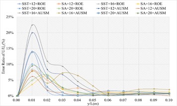
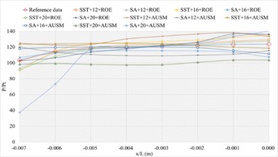
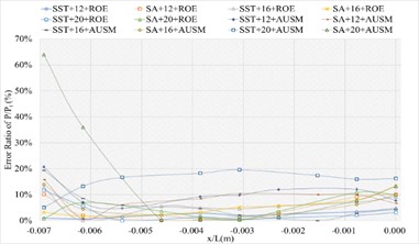
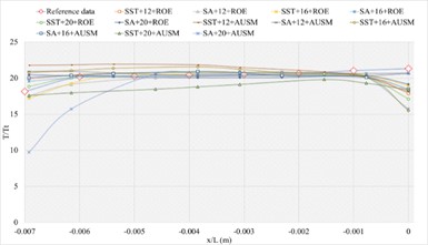
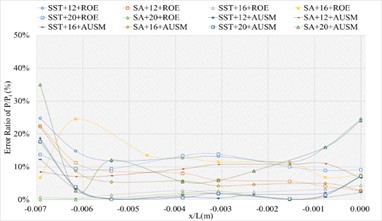
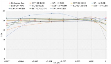
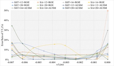
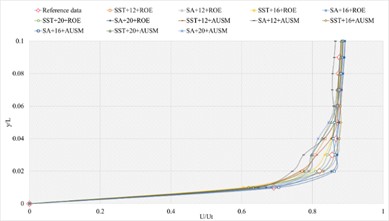
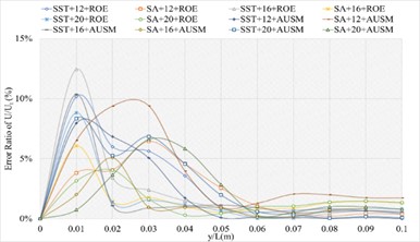
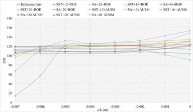
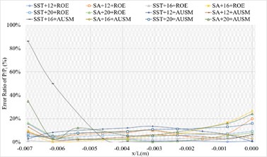
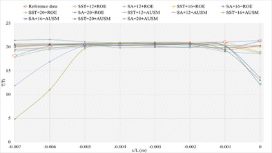
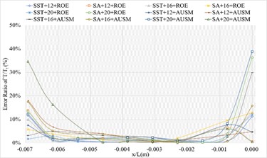
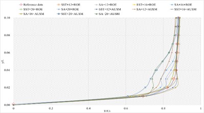
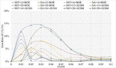
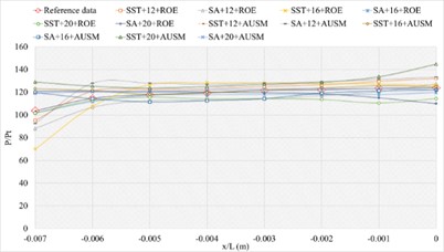
The corresponding numerical results and distributions of $P / P_{t}$ , $T / T_{t}$ and $U / U_{t}$ are shown in Tables 17-19 and Fig. 14. Table 23 provides the mean error ratios under different simulation configurations. From the aspect of far field distance, the minimum values are 2.866 %, 2.047 %, and 3.376 % in order. From the aspect of turbulence model, the most favorable outcome for SST is 3.264 %, while that of SA is 2.047 %. For the two flux types, the finest value of ROE is 2.047 % and that of AUSM is 3.264 %. In conclusion, the SA+16L configuration, combined with ROE has achieved the minimum mean error ratio. Compared with other simulation configurations, the corresponding accuracy improvements are 36.670 %, 65.361 %, 28.590 %, 56.800 %, 66.338 %, 37.299 %, 37.549 %, 54.702 %, 64.219 %, 46.723 %, and 39.367 %, respectively.

Table 17Numerical results of P/Pt of sharp trailing edge based on definition formula (200 points) adopting two turbulence models, three far field distances and two flux types

NACA0012 models		$x$ / $L$ (m) and $P$ / $P_{t}$ wind tunnel data ( $P$ / $P_{t}$ numerical data)
		–0.007	–0.006	–0.005	–0.004	–0.003	–0.002	–0.001	0
		103.6285	114.5508	117.8656	119.3983	121.7447	122.1036	123.3942	123.8330
SST+12 $L$	ROE	95.2490	121.0420	122.3321	123.1870	124.9979	126.5275	129.6336	132.2661
SST+12 $L$	AUSM	129.6510	127.9943	126.6424	127.8131	128.1751	127.3835	125.5274	122.0080
SA+12 $L$	ROE	88.1361	106.7947	112.6416	113.1061	114.1654	117.0814	120.5537	127.4284
SA+12 $L$	AUSM	92.6078	127.9824	128.0527	127.0169	128.0833	129.2793	131.2632	133.4659
SST+16 $L$	ROE	70.0133	107.5888	126.7207	128.4036	128.3239	127.5474	127.2913	126.4086
SST+16 $L$	AUSM	123.2248	121.5232	118.3046	119.8646	121.7615	123.6976	125.7666	124.9552
SA+16 $L$	ROE	101.5952	111.8097	117.2720	117.7607	118.0276	118.0976	117.8711	119.7389
SA+16 $L$	AUSM	119.8220	114.3523	111.4593	112.6008	114.4394	119.3344	121.2641	122.1085
SST+20 $L$	ROE	101.8103	112.8437	115.7255	114.2609	114.3502	113.7401	110.6038	114.4976
SST+20 $L$	AUSM	129.1016	125.3428	123.7512	125.0469	126.9627	128.7558	133.7061	144.7895
SA+20 $L$	ROE	121.1185	120.9658	120.7203	120.3242	119.6663	118.7319	115.1396	110.0396
SA+20 $L$	AUSM	119.1405	120.4283	120.6966	122.0053	122.8732	123.2574	123.3283	121.9717

Table 18Numerical results of T/Tt of sharp trailing edge based on definition formula (200 points) adopting two turbulence models, three far field distances and two flux types

NACA0012 models		$x$ / $L$ (m) and $T$ / $T_{t}$ wind tunnel data ( $T$ / $T_{t}$ numerical data)
		–0.007	–0.006	–0.005	–0.004	–0.003	–0.002	–0.001	0
		18.152	20.190	20.284	20.427	20.521	20.664	21.043	21.327
SST+12 $L$	ROE	16.551	19.384	20.448	20.622	20.666	20.651	20.270	18.759
SST+12 $L$	AUSM	20.727	21.044	21.272	21.549	21.585	20.283	19.882	16.591
SA+12 $L$	ROE	17.981	19.476	20.274	20.411	20.527	20.688	20.812	20.568
SA+12 $L$	AUSM	14.238	19.106	20.805	20.829	20.869	20.741	20.767	20.866
SST+16 $L$	ROE	11.797	17.598	20.550	21.057	21.280	21.064	20.717	20.642
SST+16 $L$	AUSM	19.688	20.028	20.234	20.448	20.627	20.889	21.297	17.054
SA+16 $L$	ROE	19.274	19.891	20.245	20.439	20.516	20.648	20.695	20.217
SA+16 $L$	AUSM	20.448	20.500	20.518	20.514	20.404	20.293	20.064	19.781
SST+20 $L$	ROE	17.608	18.326	18.700	18.845	19.056	19.702	19.834	19.830
SST+20 $L$	AUSM	20.882	21.048	21.204	21.310	21.056	20.465	20.164	20.226
SA+20 $L$	ROE	20.707	20.751	20.773	20.766	20.769	20.760	20.145	19.683
SA+20 $L$	AUSM	18.929	19.318	19.726	19.914	20.181	20.654	20.752	17.893

Table 19Numerical results of U/Ut of sharp trailing edge based on definition formula (200 points) adopting two turbulence models, three far field distances and two flux types

NACA0012 models		$y$ / $L$ (m) at $x$ / $L$ = 0.95 m and $U$ / $U_{t}$ wind tunnel data ( $U$ / $U_{t}$ numerical data)
		0.01	0.02	0.03	0.04	0.05	0.06	0.07	0.08	0.09	0.1
		0.6907	0.8199	0.8556	0.8667	0.8705	0.8711	0.8740	0.8746	0.8771	0.8801
SST+12 $L$	ROE	0.6634	0.8368	0.8552	0.8629	0.8684	0.8730	0.8766	0.8808	0.8844	0.8866
SST+12 $L$	AUSM	0.6104	0.8114	0.8678	0.8737	0.8693	0.8687	0.8720	0.8782	0.8843	0.8877
SA+12 $L$	ROE	0.7054	0.8717	0.8779	0.8770	0.8751	0.8748	0.8762	0.8796	0.8837	0.8866
SA+12 $L$	AUSM	0.7205	0.8669	0.8665	0.8694	0.8760	0.8803	0.8825	0.8848	0.8872	0.8887
SST+16 $L$	ROE	0.6519	0.8574	0.8755	0.8749	0.8743	0.8756	0.8784	0.8830	0.8877	0.8905
SST+16 $L$	AUSM	0.6017	0.8144	0.8655	0.8726	0.8749	0.8764	0.8785	0.8823	0.8863	0.8889
SA+16 $L$	ROE	0.7092	0.8739	0.8681	0.8692	0.8746	0.8796	0.8830	0.8863	0.8891	0.8908
SA+16 $L$	AUSM	0.6745	0.8656	0.8790	0.8745	0.8693	0.8685	0.8698	0.8734	0.8780	0.8816
SST+20 $L$	ROE	0.6450	0.8527	0.8731	0.8746	0.8760	0.8791	0.8821	0.8857	0.8889	0.8909
SST+20 $L$	AUSM	0.5981	0.7864	0.8374	0.8651	0.8692	0.8700	0.8726	0.8775	0.8826	0.8858
SA+20 $L$	ROE	0.6860	0.8558	0.8776	0.8731	0.8713	0.8733	0.8767	0.8819	0.8868	0.8898
SA+20 $L$	AUSM	0.7078	0.7781	0.8094	0.8215	0.8393	0.8573	0.8664	0.8720	0.8762	0.8786

Fig. 14The numerical result and error ratio distributions of P/Pt, T/Tt and U/Ut of sharp trailing edge based on definition formula (200 points)

a) Numerical result distribution of $P / P_{t}$ of the sharp trailing edge based on definition formula (200 points)

b) Error ratio distribution of $P / P_{t}$ of the sharp trailing edge based on definition formula (200 points)

c) Numerical result distribution of $T / T_{t}$ of the sharp trailing edge based on definition formula (200 points)

d) Error ratio distribution of $T / T_{t}$ of the sharp trailing edge based on definition formula (200 points)

e) Numerical result distribution of $U / U_{t}$ of the sharp trailing edge based on definition formula (200 points)

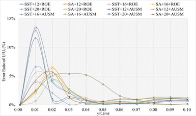
f) Error ratio distribution of $U / U_{t}$ of the sharp trailing edge based on definition formula (200 points)

3.1.6. Definition formula adopting 400 points

The corresponding numerical results and distributions of $P / P_{t}$ , $T / T_{t}$ and $U / U_{t}$ are shown in Tables 20-22 and Fig. 15. Table 23 provides the calculated mean error ratios under different simulation configurations. From the aspect of far field distance, the minimum values are 4.136 %, 2.460 %, and 2.454 % in order. From the aspect of turbulence model, the most favorable outcome for SST is 2.454 %, while that of SA is 3.482 %. For the two flux types, the finest value of ROE is 2.454 % and that of AUSM is 3.482 %. In conclusion, the SST+20 $L$ configuration, combined with ROE has achieved the minimum mean error ratio. Compared with other simulation configurations, the corresponding accuracy improvements are 40.670 %, 80.420 %, 56.911 %, 71.324 %, 0.240 %, 61.911 %, 33.899 %, 29.537 %, 40.134 %, 36.977 %, and 59.327 %, respectively.

Table 20Numerical results of P/Pt of sharp trailing edge based on definition formula (400 points) adopting two turbulence models, three far field distances and two flux types

NACA0012 models		$x$ / $L$ (m) and $P$ / $P_{t}$ wind tunnel data ( $P$ / $P_{t}$ numerical data)
		–0.007	–0.006	–0.005	–0.004	–0.003	–0.002	–0.001	0
		103.6285	114.5508	117.8656	119.3983	121.7447	122.1036	123.3942	123.8330
SST+12 $L$	ROE	121.5352	121.5892	121.8436	122.3692	122.4129	122.2378	116.3225	108.3289
SST+12 $L$	AUSM	104.5392	104.3224	104.0669	103.6346	103.5846	103.5758	98.7789	94.0892
SA+12 $L$	ROE	120.7982	120.4667	120.3445	119.5408	117.6898	114.7833	100.4419	102.2569
SA+12 $L$	AUSM	106.9614	106.0633	105.1678	103.4016	102.6120	101.9376	101.4844	103.5008
SST+16 $L$	ROE	103.1487	114.1292	119.7196	122.8894	124.0935	125.0836	127.5916	129.4911
SST+16 $L$	AUSM	119.4194	119.4679	118.3171	116.7076	114.0483	110.7948	107.6613	109.6274
SA+16 $L$	ROE	84.7344	105.5092	115.0007	116.0551	119.1564	123.3079	135.0119	138.4577
SA+16 $L$	AUSM	115.7716	116.3642	117.5177	118.0496	118.5284	119.1038	118.8542	116.6833
SST+20 $L$	ROE	101.7360	113.5344	119.1353	122.2907	123.5090	124.5382	126.9285	128.7087
SST+20 $L$	AUSM	111.4175	120.3351	118.6102	120.8620	125.6442	130.3150	137.6943	143.5232
SA+20 $L$	ROE	85.6777	105.7869	113.6548	114.4745	117.0368	120.6551	134.5757	138.7417
SA+20 $L$	AUSM	86.0844	105.3288	117.5366	116.7220	118.1160	123.6655	136.1005	146.2670

Table 21Numerical results of T/Tt of sharp trailing edge based on definition formula (400 points) adopting two turbulence models, three far field distances and two flux types

NACA0012 models		$x$ / $L$ (m) and $T$ / $T_{t}$ wind tunnel data ( $T$ / $T_{t}$ numerical data)
		–0.007	–0.006	–0.005	–0.004	–0.003	–0.002	–0.001	0
		18.152	20.190	20.284	20.427	20.521	20.664	21.043	21.327
SST+12 $L$	ROE	20.476	20.586	20.682	20.862	20.944	20.889	20.056	18.964
SST+12 $L$	AUSM	19.928	20.157	20.330	20.269	19.400	16.884	8.214	3.902
SA+12 $L$	ROE	20.513	20.606	20.155	19.781	19.622	19.593	19.235	18.366
SA+12 $L$	AUSM	18.219	18.129	18.075	18.023	18.011	18.089	18.158	16.021
SST+16 $L$	ROE	19.882	20.374	20.645	20.770	20.751	20.675	20.176	18.464
SST+16 $L$	AUSM	21.466	21.187	20.172	19.808	19.637	19.458	19.065	14.682
SA+16 $L$	ROE	17.053	18.914	20.053	20.139	20.244	20.500	20.609	20.531
SA+16 $L$	AUSM	20.506	20.677	20.858	21.126	21.139	20.820	20.126	19.176
SST+20 $L$	ROE	19.831	20.385	20.670	20.797	20.776	20.697	20.190	18.259
SST+20 $L$	AUSM	18.831	19.597	20.131	20.380	20.680	20.935	21.276	20.721
SA+20 $L$	ROE	17.312	19.017	19.999	20.080	20.182	20.470	20.599	20.551
SA+20 $L$	AUSM	17.093	18.685	19.730	19.768	19.813	19.906	19.975	12.296

Table 22Numerical results of U/Ut of sharp trailing edge based on definition formula (400 points) adopting two turbulence models, three far field distances and two flux types

NACA0012 models		$y$ / $L$ (m) at $x$ / $L$ = 0.95 m and $U$ / $U_{t}$ wind tunnel data ( $U$ / $U_{t}$ numerical data)
		0.01	0.02	0.03	0.04	0.05	0.06	0.07	0.08	0.09	0.1
		0.6907	0.8199	0.8556	0.8667	0.8705	0.8711	0.8740	0.8746	0.8771	0.8801
SST+12 $L$	ROE	0.6754	0.8645	0.8788	0.8759	0.8754	0.8778	0.8805	0.8837	0.8867	0.8885
SST+12 $L$	AUSM	0.6956	0.8018	0.7984	0.8265	0.8641	0.8782	0.8813	0.8818	0.8821	0.8823
SA+12 $L$	ROE	0.7301	0.8741	0.8743	0.8742	0.8761	0.8785	0.8806	0.8834	0.8863	0.8880
SA+12 $L$	AUSM	0.7055	0.8441	0.8732	0.8773	0.8712	0.8689	0.8696	0.8732	0.8779	0.8809
SST+16 $L$	ROE	0.6532	0.8335	0.8533	0.8617	0.8677	0.8725	0.8763	0.8805	0.8844	0.8867
SST+16 $L$	AUSM	0.5980	0.8120	0.8621	0.8703	0.8747	0.8769	0.8778	0.8797	0.8828	0.8850
SA+16 $L$	ROE	0.6972	0.8703	0.8708	0.8670	0.8689	0.8743	0.8789	0.8833	0.8870	0.8892
SA+16 $L$	AUSM	0.7106	0.8780	0.8699	0.8702	0.8764	0.8799	0.8816	0.8844	0.8878	0.8900
SST+20 $L$	ROE	0.6505	0.8288	0.8516	0.8607	0.8669	0.8721	0.8762	0.8808	0.8850	0.8875
SST+20 $L$	AUSM	0.6226	0.7503	0.7943	0.8283	0.8415	0.8480	0.8542	0.8626	0.8699	0.8743
SA+20 $L$	ROE	0.6937	0.8678	0.8749	0.8770	0.8783	0.8798	0.8816	0.8844	0.8877	0.8898
SA+20 $L$	AUSM	0.7392	0.8062	0.8433	0.8700	0.8778	0.8755	0.8724	0.8716	0.8730	0.8741

Fig. 15The numerical result and error ratio distributions of P/Pt, T/Tt and U/Ut of sharp trailing edge based on definition formula (400 points)

a) Numerical result distribution of $P / P_{t}$ of the sharp trailing edge based on definition formula (400 points)

b) Error ratio distribution of $P / P_{t}$ of the sharp trailing edge based on definition formula (400 points)

c) Numerical result distribution of $T / T_{t}$ of the sharp trailing edge based on definition formula (400 points)

d) Error ratio distribution of $T / T_{t}$ of the sharp trailing edge based on definition formula (400 points)

e) Numerical result distribution of $U / U_{t}$ of the sharp trailing edge based on definition formula (400 points)

f) Error ratio distribution of $U / U_{t}$ of the sharp trailing edge based on definition formula (400 points)

Table 23The mean error ratios for the six NACA0012 models under different simulation configurations

Simulation configuration	NACA0012 models	ROE (%)				AUSM (%)
Simulation configuration	NACA0012 models	$P / P_{t}$	$T / T_{t}$	$U / U_{t}$	Total mean error ratio of ( $P / P_{t}$ , $T / T_{t}$ , $U / U_{t}$ )	$P / P_{t}$	$T / T_{t}$	$U / U_{t}$	Total mean error ratio of ( $P / P_{t}$ , $T / T_{t}$ , $U / U_{t}$ )
SST+12L	Blunt	1.968	4.523	1.598	2.696	8.939	5.909	4.072	6.307
	NACA4	2.276	3.962	1.035	2.424	10.415	8.540	4.376	7.777
	Definition formula (132 points)	16.132	9.272	2.950	9.451	4.316	2.877	2.214	3.136
	Definition formula (264 points)	3.437	3.811	1.230	2.826	7.955	2.814	0.697	3.822
	Definition formula (200 points)	4.860	3.881	0.955	3.232	8.019	7.942	1.766	5.909
	Definition formula (400 points)	6.025	4.722	1.660	4.136	13.597	22.172	1.826	12.532
SST+16L	Blunt	2.197	4.485	1.532	2.738	8.155	13.631	5.249	9.012
	Naca4	6.228	3.245	2.357	3.943	5.962	8.189	2.072	5.408
	Definition formula (132 points)	2.137	4.212	1.569	2.640	2.779	6.139	1.781	3.566
	Definition formula (264 points)	2.621	4.002	1.652	2.758	18.768	17.841	1.622	12.744
	Definition formula (200 points)	8.584	7.830	1.827	6.080	3.738	4.059	1.996	3.264
	Definition formula (400points)	2.209	4.077	1.093	2.460	7.746	9.685	1.893	6.442
SST+20L	Blunt	5.272	3.356	1.681	3.436	9.471	6.024	2.860	6.119
	NACA4	3.148	4.142	2.276	3.189	15.305	7.999	2.384	8.562
	Definition formula (132 points)	11.002	4.356	1.612	5.657	4.140	4.644	2.830	3.871
	Definition formula (264 points)	6.034	2.755	1.560	3.449	9.670	8.474	6.990	8.378
	Definition formula (200 points)	5.024	6.543	1.988	4.518	9.843	5.132	2.186	5.720
	Definition formula (400 points)	2.057	4.222	1.082	2.454	6.480	1.713	4.103	4.099
SA+12L	Blunt	24.038	24.609	2.394	17.014	3.619	5.559	1.145	3.441
	NACA4	4.422	2.164	1.901	2.829	8.525	3.545	1.404	4.491
	Definition formula (132 points)	8.581	9.701	2.410	6.897	8.912	6.314	3.912	6.379
	Definition formula (264 points)	8.416	3.388	1.728	4.511	5.190	5.030	4.085	4.768
	Definition formula (200 points)	5.871	1.176	1.552	2.866	7.828	4.626	1.759	4.738
	Definition formula (400 points)	8.663	6.363	2.057	5.694	12.650	12.065	0.954	8.556
SA+16L	Blunt	3.519	4.375	1.980	3.292	5.893	6.107	3.625	5.209
	NACA4	5.325	5.244	1.610	4.060	5.116	4.569	1.707	3.797
	Definition formula (132 points)	11.850	8.200	1.664	7.238	7.323	5.833	1.261	4.805
	Definition formula (264 points)	8.819	4.448	2.921	5.396	6.809	8.172	1.229	5.403
	Definition formula (200 points)	2.543	1.859	1.738	2.047	4.789	3.754	1.289	3.277
	Definition formula (400 points)	6.962	2.857	1.317	3.712	3.660	4.980	1.806	3.482
SA+20L	Blunt	6.399	2.696	2.007	3.701	7.272	1.680	2.220	3.724
	Naca4	4.685	4.283	1.728	3.565	15.453	9.744	2.061	9.086
	Definition formula (132 points)	1.760	5.580	1.586	2.975	13.734	7.500	2.340	7.858
	Definition formula (264 points)	5.111	7.582	1.259	4.651	13.734	7.500	5.673	8.969
	Definition formula (200 points)	5.997	4.323	1.206	3.842	3.514	4.132	2.481	3.376
	Definition formula (400 points)	7.353	2.735	1.592	3.893	7.522	9.223	1.353	6.033

3.2. Discussion

3.2.1. Cell Reynolds number and aspect ratio

The cell Reynolds number ( $R_{c e l l}$ ) of near-wall mesh cells close to the shock are crucial in affecting the numerical error ratio. Taking blunt cylinder as the characteristic object, Ref. [30] points out that the $R_{c e l l}$ value of the near shock wave grid cells should be no less than 8. Moreover, Ref. [31] shows that the aspect ratio of wall cells near the shock significantly impacts simulation performance. In this paper, based on the existing research, to investigate the influences of $R_{c e l l}$ and aspect ratio of the near shock wave wall grid cells with NACA0012 as the characteristic object, the $R_{c e l l}$ of near shock wave wall grid cells is first analyzed while keeping the total mesh number unchanged. Based on the optimal simulation configuration conclude in Section 3.1, we apply three $R_{c e l l}$ values of 16, 8, and 4 and the related $y^{+}$ and $y_{H}$ values are (0.3 1.4e-5 m), (0.15 7e-6 m), and (0.08 3.5e-6 m). Three numerical simulations are performed and the corresponding mean error ratios of ( $P / P_{t}$ , $T / T_{t}$ , $U / U_{t}$ ) are (2.54 % 1.86 % 1.74 %), (2.62 % 2.09 % 2.01 %), and (6.38 % 4.77 % 2.47 %) respectively, as shown in Table 24. Therefore, the optimal results are obtained by $R_{c e l l}$ value of 16. Next, to study the influence of aspect ratio on numerical accuracy, we made changes to the wall cells' aspect ratio near the shock while keeping the following conditions constant: (1) The total number of mesh cells remained the same. (2) The cell Reynolds number remained the same. (3) The aspect ratio changes were made only in small wall regions near the shock. The aspect ratio value of the near-wall mesh close to the shock at the optimal $R_{c e l l}$ value is 380, through double and halve operations we select four aspect ratio values of 760, 380, 190, and 95. Another four simulations are executed and the corresponding comparison of error ratios are described in Table 25. When the aspect ratio is 380, the minimum simulation result is achieved, which is 2.05 %. Then with the further increase of the aspect ratio, the error ratio is also increased. Compared with the other three aspect ratios, the accuracy improvements are 63.97 %, 46.75 % and 65.37 %. In summarize, unlike the suggestions proposed in the existing research characterized by blunt cylinder, the suitable value for $R_{c e l l}$ characterized by NACA0012 should be no smaller than 16, reducing this value will decrease numerical accuracy. Similar situation applies to the aspect ratio, smaller value would not lead to better numerical calculation and the recommended value is 380.

Table 24Comparison of numerical error ratios under three cell Reynolds numbers

Cell Reynolds number	$P / P_{t}$	$T / T_{t}$	$U / U_{t}$	Mean error ratio
16 ( $y^{+} =$ 0.3)	2.54 %	1.86 %	1.74 %	2.05 %
8 ( $y^{+} =$ 0.15)	2.62 %	2.09 %	2.01 %	2.24 %
4 ( $y^{+} =$ 0.08)	6.38 %	4.77 %	2.47 %	4.54 %

Table 25Comparison of numerical error ratios under four aspect ratios

Aspect ratio	$P / P_{t}$	$T / T_{t}$	$U / U_{t}$	Mean error ratio	Accuracy improvement among aspect ratios
95	4.78 %	6.26 %	6.04 %	5.69 %	63.97 %
190	4.35 %	3.49 %	3.71 %	3.85 %	46.75 %
380	2.54 %	1.86 %	1.74 %	2.05 %	0.00 %
760	8.56 %	4.07 %	5.13 %	5.92 %	65.37 %

3.3. Trailing edge shape and modeling method

Fig. 16 depicts the optimal numerical error ratios comparison among six NACA0012 model, where the left ordinate indicates the numerical error ratio displayed in a column graph, and the right ordinate indicates the accuracy improvement displayed in a line chart. Fig. 17 adopts the same settings. From the aspect of trailing edge shape, based on Airfoil tools, the designed blunt trailing edge’s numerical performance is worse than that of other types of sharp trailing edge (the sharp trailing edge adopting 264 data points definition formula is excluded), with the numerical accuracy decreasing by 11.41 %, 2.14 %, 31.73 % and 9.88 %, respectively. For the three modeling methods, the corresponding finest numerical error ratio is 2.7 %, 2.42 % and 2.05 % in order. It is worth noting that although the smallest error ratio could be obtained using the definition formula of 200 data points, the numerical results of the airfoil designed based on NACA4 are better in other cases. The correlation between the number and source of data points of the definition formula and the calculation precision is further analyzed. Airfoil tools offers 132 data points, with the data points increasing to 264, the numerical accuracy decreases by 4.55 %. NACA4 offers 200 data points, and the increase in data amount also results in a decrease in numerical accuracy of 19.71 %. When using 200 and 400 data points, the optimal numerical error ratios are 2.05 % and 2.454 %, respectively. These ratios are superior to those based on 132 and 264 data points. In summarize, unlike existing research conclusions [28-29], firstly, there exists a significant decrease in accuracy may occur due to an incorrect shape of the trailing edge in NACA0012, the maximum value of which is up to 31.73 %. The sharp trailing edge is recommended, and the number of data points adopted for NACA0012 modeling is the key to the selection of definition formula or NACA4. Secondly, the performance of data points provided by NACA4 is superior to that provided by Airfoil tools, and there is no positive correlation between the data points number and the calculation accuracy. Lastly, it is recommended to use the definition formula that utilizes NACA4's 200 points to design the sharp trailing edge shape.

3.3.1. Far field distance, turbulence model and flux type

Fig. 17 depicts the optimal numerical error ratios comparison among far field distances, turbulence models and flux types. As to the far field distance, the numerical precision increases by 15.42 %, with the far field distance increasing from 12 $L$ to 16 $L$ . But with the far field distance reaching 20L, the simulation precision declines by 19.88 %. When considering the turbulence model, the SST k-omega model proves to be more effective than the SA model at far field distances of 12 $L$ and 20 $L$ .

Fig. 16The optimal numerical error ratio comparison among six NACA0012 models

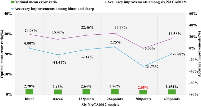
Fig. 17The optimal numerical error ratio comparison among far field distances, turbulence models, and flux types

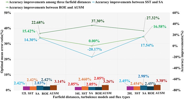
The numerical accuracy is also enhanced by 14.3 % and 17.54 %, respectively. However, at 16 $L$ far field distance, the SA model obtains the smallest error ratio. From the perspective of flux type, compared with AUSM, the numerical performance of ROE is better. The maximum increase is 37.3 %, and the minimum increase is 22.68 %. In summary, unlike the research conclusions in Ref. [29], firstly, the increase in far field distance is not necessarily positively correlated with the calculation accuracy. Keeping 16 $L$ far field distance is recommended. Secondly, the turbulence model selection is associated with the distance of the far field, and according to the ideal value of far field distance, it is recommended to prioritize the SA model. Lastly, the ROE flux type is preferred. Therefore, under hypersonic conditions, the preferred simulation configurations of NACA0012 are the sharp trailing edge (definition formula adopting 200 data points) + 16 $L$ + SA turbulence model + ROE, with the $R_{c e l l}$ and aspect ratio values of near-wall mesh near the shock are 16 and 380.

4. Simulation scheme and aerodynamic environment prediction

To simplify the analysis, it is assumed that the flight speed is increased uniformly, and the acceleration process could be completed instantaneously without considering the influence of fuel and engine performance. According to the flight path described in Fig. 1, the flight process is divided into sub-phases in seconds. Maintain a constant speed within each sub-phase and complete the acceleration process instantly when entering the next sub-phase. The hypersonic conditions can be divided into 11 sub-phases, which first undergo the accelerated flight for 10 s (hypersonic 1-hypersonic 10), and then maintain the steady flight at the same height and speed when the flow velocity reaches 6.5 Ma (hypersonic 11). According to the conclusion drawn from the detailed discussion in Section 3.2, an effective simulation scheme for the aerodynamic environment prediction under hypersonic conditions characterized by NACA0012 is shown in Table 26. The applied computational external flow field is shown in Fig. 3(a).

Table 26The simulation scheme under hypersonic conditions characterized by NACA0012

Simulation scheme	Values
Hypersonic conditions	hypersonic1 $M$ = 5.100 $P_{t}$ = 3467 Pa $T_{t}$ = 219.65 K $μ$ = 1.438e-5 Pa·s $ρ$ = 0.055 kg/m³
	hypersonic2 $M$ = 5.250 $P_{t}$ = 3218 Pa $T_{t}$ = 220.15 K $μ$ = 1.441e-5 Pa·s $ρ$ = 0.051 kg/m³
	hypersonic3 $M$ = 5.400 $P_{t}$ = 2972 Pa $T_{t}$ = 220.65 K $μ$ = 1.444e-5 Pa·s $ρ$ = 0.047 kg/m³
	hypersonic4 $M$ = 5.550 $P_{t}$ = 2753 Pa $T_{t}$ = 221.15 K $μ$ = 1.446e-5 Pa·s $ρ$ = 0.043 kg/m³
	hypersonic5 $M$ = 5.700 $P_{t}$ = 2549 Pa $T_{t}$ = 221.65 K $μ$ = 1.449e-5 Pa·s $ρ$ = 0.040 kg/m³
	hypersonic6 $M$ = 5.850 $P_{t}$ = 2361 Pa $T_{t}$ = 222.15 K $μ$ = 1.452e-5 Pa·s $ρ$ = 0.037 kg/m³
	hypersonic7 $M$ = 6.000 $P_{t}$ = 2188 Pa $T_{t}$ = 222.65 K $μ$ = 1.454e-5 Pa·s $ρ$ = 0.034 kg/m³
	hypersonic8 $M$ = 6.125 $P_{t}$ = 1880 Pa $T_{t}$ = 223.54 K $μ$ = 1.459e-5 Pa·s $ρ$ = 0.029 kg/m³
	hypersonic9 $M$ = 6.250 $P_{t}$ = 1610 Pa $T_{t}$ = 224.53 K $μ$ = 1.465e-5 Pa·s $ρ$ = 0.025 kg/m³
	hypersonic10 $M$ = 6.375 $P_{t}$ = 1390 Pa $T_{t}$ = 225.52 K $μ$ = 1.470e-5 Pa·s $ρ$ = 0.021 kg/m³
	hypersonic11 $M$ = 6.500 $P_{t}$ = 1197 Pa $T_{t}$ = 226.51 K $μ$ = 1.475e-5 Pa·s $ρ$ = 0.018 kg/m³
Grid strategy	hypersonic1 $C_{a i r}$ = 297 m/s $U_{t}$ = 1516 m/s $y^{+} =$ 0.3 ( $R_{c e l l} =$ 16) $y_{H} =$ 2e-6 m as ratio = 380
	hypersonic2 $C_{a i r}$ = 298 m/s $U_{t}$ = 1562 m/s $y^{+} =$ 0.3 ( $R_{c e l l} =$ 16) $y_{H} =$ 2e-6 m as ratio = 380
	hypersonic3 $C_{a i r}$ = 298 m/s $U_{t}$ = 1608 m/s $y^{+} =$ 0.3 ( $R_{c e l l} =$ 16) $y_{H} =$ 2e-6 m as ratio = 380
	hypersonic4 $C_{a i r}$ = 298 m/s $U_{t}$ = 1655 m/s $y^{+} =$ 0.3 ( $R_{c e l l} =$ 16) $y_{H} =$ 2e-6 m as ratio = 380
	hypersonic5 $C_{a i r}$ = 299 m/s $U_{t}$ = 1702 m/s $y^{+} =$ 0.3 ( $R_{c e l l} =$ 16) $y_{H} =$ 2e-6 m as ratio = 380
	hypersonic6 $C_{a i r}$ = 299 m/s $U_{t}$ = 1748 m/s $y^{+} =$ 0.3 ( $R_{c e l l} =$ 16) $y_{H} =$ 2e-6 m as ratio = 380
	hypersonic7 $C_{a i r}$ = 299 m/s $U_{t}$ = 1795 m/s $y^{+} =$ 0.3 ( $R_{c e l l} =$ 16) $y_{H} =$ 2e-6 m as ratio = 380
	hypersonic8 $C_{a i r}$ = 300 m/s $U_{t}$ = 1836 m/s $y^{+} =$ 0.3 ( $R_{c e l l} =$ 16) $y_{H} =$ 2e-6 m as ratio = 380
	hypersonic9 $C_{a i r}$ = 300 m/s $U_{t}$ = 1878 m/s $y^{+} =$ 0.3 ( $R_{c e l l} =$ 16) $y_{H} =$ 2e-6 m as ratio = 380
	hypersonic10 $C_{a i r}$ = 301m/s $U_{t}$ = 1920 m/s $y^{+} =$ 0.3 ( $R_{c e l l} =$ 16) $y_{H} =$ 2e-6 m as ratio = 380
	hypersonic11 $C_{a i r}$ = 302m/s $U_{t}$ = 1961 m/s $y^{+} =$ 0.3 ( $R_{c e l l} =$ 16) $y_{H} =$ 2e-6 m as ratio = 380
Numerical method	Turbulence model	Spalart-allmaras: turbulent viscosity ratio 1
	Materials	Density: ideal-gas; viscosity: sutherland law; Cp (j/kg-k): 1006.43
	Solver	Density-based solver adopting ROE flux type
		Gradient: least-squares cell-based; Flow: second-order upwind
		Modified turbulent viscosity: second-order upwind

Fig. 18The aerodynamic environment prediction under hypersonic condition characterized by NACA0012

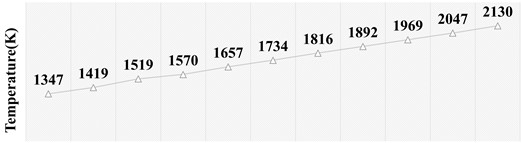
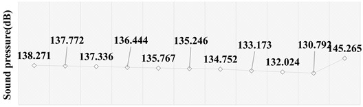
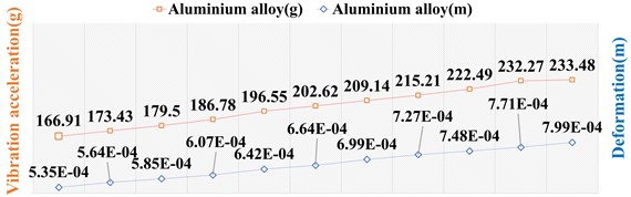
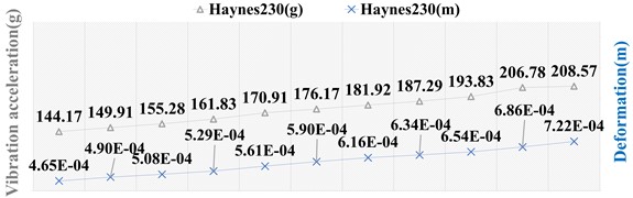
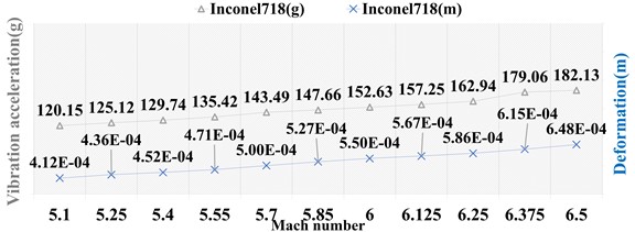
The aerodynamic environment prediction characterized by NACA0012 under hypersonic conditions is shown in Fig. 18. Firstly, the change of aerodynamic heat is analyzed. The maximum aerodynamic heat rises to 2130 K (1856.85 °C), which was consistent with the aerodynamic heat descriptions in Refs. [40], [41]. The temperature increases by 847 °C, with an average temperature change rate of about 77 °C/s. With the flow velocity increases, the aerodynamic thermal variation amplitude and average change rate are higher. The temperature extreme point is in front of the leading edge, and the temperature at the leading edge is higher than that at the trailing edge. Then, the aerodynamic sound pressure is analyzed. The minimum and maximum sound pressure levels are 130.8 dB and 145.3 dB. Fig. 19 demonstrates the distribution of frequencies in acoustic signals. Only in hypersonic 3 the middle and high frequencies above 100 Hz have contribution to the sound signal, and the middle and high frequencies in other substages are basically negligible. In general, it is the low-frequency signal within 100 Hz dominate under hypersonic conditions. Finally, the vibration analysis is conducted, and we first need to ascertain the material composition of the NACA0012 airfoil. The X43 A and X51 A are representative scramjet-propelled hypersonic vehicles, with the airfoil of the former utilizing haynes230 and that of the latter employing inconel718. In this paper, we adopt these two materials and the standard aluminium to analyze the influence of materials on vibration. Fig. 18 shows that Inconel718 has better compression and temperature resistance and could withstand relatively minimum average vibration acceleration and deformation amplitude. The NACA0012 with Inconel718 alloy experiences a maximum vibration acceleration ranges of 120 g to 182 g. Compared to aluminium alloy, the adoption of Inconel718 results in a vibration/deformation optimization range of 21.99 % to 28.02 % and 18.90 % to 22.99 %, respectively. As the flow velocity and temperature increase, both vibration acceleration and deformation also increase, leading to a decrease in the optimization degree achieved by Inconel718. Compared with aluminium alloy, Inconel718 still could bring a minimum optimization amplitude of 21.99 % for vibration acceleration and 18.90 % for deformation. The utilization of novel materials can yield considerable enhancements in structural reliability. To sum up, the scramjet-propelled vehicle encounters significant aerodynamic challenges under hypersonic conditions during the flight.

Fig. 19Distribution of acoustic signals of different frequencies under hypersonic conditions characterized by NACA0012

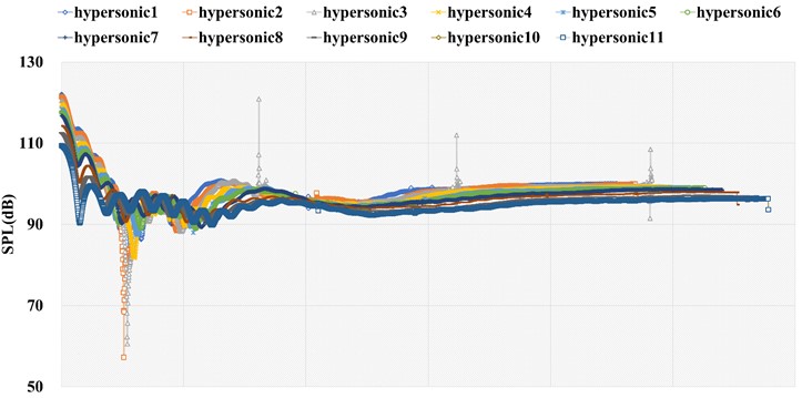
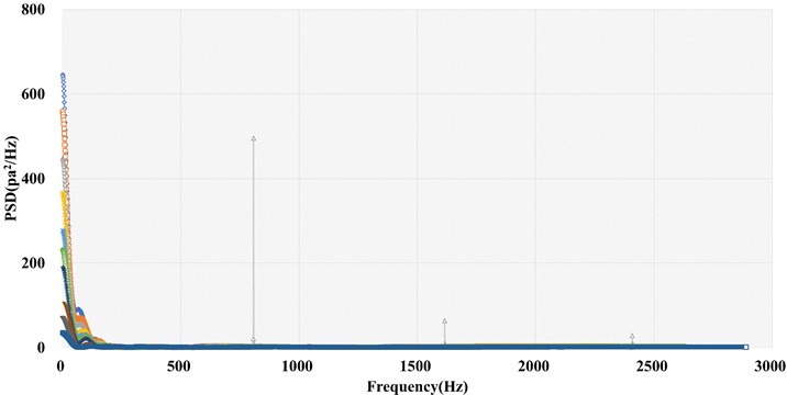
5. Conclusions

Aiming at the insufficient research on the aerodynamic environment prediction of scramjet-propelled vehicles characterized by NACA0012 under hypersonic conditions, in this paper, based on the wind tunnel experimental data, a comprehensive analysis is performed to study the influences of key simulation parameters on numerical accuracy and an effective simulation scheme for aerodynamic environment prediction under hypersonic conditions characterized by NACA0012 is proposed. In Section 2, we introduce the adopted grid strategy and numerical method. In Section 3, based on six NACA0012 models, three far field distances, two turbulence models, and two flux types, with additional three cell Reynolds numbers, and four aspect ratios, CFD simulations are conducted and the internal relationship between simulation parameters and numerical accuracy is discussed by comparing the numerical results with the wind tunnel data. Characterized by NACA0012, the optimal simulation configuration under hypersonic conditions is derived and the corresponding aerodynamic environment prediction is carried out in Section 4. Through systematic analysis, the study findings are as follows:

1) Compared with the blunt trailing edge, better numerical results could be obtained with the sharp trailing edge. It's worth noting that an incorrect sharp trailing edge modeling method could result in a higher numerical error ratio than a blunt trailing edge. Therefore, it's essential to select the sharp trailing edge modeling method with great care. Preference is given to the definition formula for designing the sharp trailing edge. The source and number of data points used by the definition formula would directly affect the numerical results. In this paper, the data points used in the definition formula are derived from Airfoil tools and NACA4, and the numerical analysis indicates that NACA4’s data points perform better. These two modeling data point sources have a negative correlation between the data points number and the numerical accuracy.

2) Unlike under incompressible conditions, the recommended values for far field distance and flux type are 16L and ROE flux type, respectively. In particular, the appropriate modified turbulent viscosity for Spalart-Allmaras turbulence model is second order upwind. Moreover, unlike taking the blunt cylinder as the characterized object, the proposed values of cell Reynolds number and aspect ratio of airfoil mesh cells close to the shock are no smaller than 16 and no larger than 380, respectively.

3) The extreme aerodynamic environments place high demands on ground environment testing. The temperature of heating device can reach 1900 ℃ and the maximum temperature rise rate can reach 77 ℃/s. The vibration table supports a maximum vibration acceleration of 182 g and the maximum sound pressure level of the sound test reverberation room reaches 145 dB, mainly containing low-frequency signals within 100 Hz. In addition, the influence of aerodynamic heat on the structural vibration increases with the increase of flow velocity, indicating thermal vibration testing should be conducted jointly during environmental testing to better evaluate the structural stability of the vehicle.

4) The utilization of advanced materials like Haynes230 and Inconel718 plays a pivotal role in enhancing structural reliability. Although the optimization efficacy of these materials diminishes with escalating flow velocity and aerodynamic heat, the growth remains considerable. Inconel718 having better compression and heat resistance performance, which is recommended for airfoil design.

5) The research conclusions proposed in this paper provide the basis for the parameter selection and simulation scheme design for predicting the extreme aerodynamic environment experienced by the hypersonic vehicle during the flight. Researchers could obtain more accurate environmental extremes, conduct more efficient structural design and ground testing, avoid redundant protection design, reduce costs, and improve efficiency.

6) The flight trajectory of hypersonic vehicle spans transonic, supersonic, high supersonic and hypersonic four stages. In this paper, we discuss the hypersonic conditions occupying over 90 % of the flight external flow field, while the other three external flow field are not investigated. To further improve the predictive accuracy of vehicle flight environment and provide more accurate numerical references for vehicle design and optimization, future research directions should be firstly to analyze the internal relationships between simulation parameters and numerical accuracy under the other three external flow fields in order, then perform a complete flight environment prediction based on the optimal simulation configurations concluded under four external flow fields.

References

B. C. Ai, Computational Aerodynamics of Near-Space Hypersonic Vehicles. Beijing: Science Press, 2020.

Search CrossRef
J. Lee and O. Rho, “Accuracy of AUSM+ scheme in hypersonic blunt body flow calculations,” in 8th AIAA International Space Planes and Hypersonic Systems and Technologies Conference, Apr. 1998, https://doi.org/10.2514/6.1998-1538

Publisher
K. Kitamura, E. Shima, Y. Nakamura, and P. L. Roe, “Evaluation of Euler fluxes for hypersonic heating computations,” AIAA Journal, Vol. 48, No. 4, pp. 763–776, Apr. 2010, https://doi.org/10.2514/1.41605

Publisher
I. Di Venuta, I. Petracci, M. Angelino, A. Boghi, and F. Gori, “Numerical simulation of mass transfer and fluid flow evolution of a rectangular free jet of air,” International Journal of Heat and Mass Transfer, Vol. 117, pp. 235–251, Feb. 2018, https://doi.org/10.1016/j.ijheatmasstransfer.2017.10.030

Publisher
F. Qu, D. Sun, and C. Yan, “A new flux splitting scheme for the Euler equations II: E-AUSMPWAS for all speeds,” Communications in Nonlinear Science and Numerical Simulation, Vol. 57, pp. 58–79, Apr. 2018, https://doi.org/10.1016/j.cnsns.2017.09.002

Publisher
F. Chen, H. Liu, and S. Zhang, “Time-adaptive loosely coupled analysis on fluid-thermal-structural behaviors of hypersonic wing structures under sustained aeroheating,” Aerospace Science and Technology, Vol. 78, pp. 620–636, Jul. 2018, https://doi.org/10.1016/j.ast.2018.05.015

Publisher
F. Qu, J. Chen, D. Sun, J. Bai, and G. Zuo, “A grid strategy for predicting the space plane’s hypersonic aerodynamic heating loads,” Aerospace Science and Technology, Vol. 86, pp. 659–670, Mar. 2019, https://doi.org/10.1016/j.ast.2019.01.049

Publisher
X. Zheng, Z. S. Liu, Y. Yang, J. C. L. Lei, and Z. X., “Research on climb-cruise global trajectory optimization for RBCC Hypersonic Vehicle,” Missiles Space Veh, Vol. 47, pp. 1–8, 2018, https://doi.org/10.7654/j.issn.1004-7182.20180201

Publisher
“Speed of Sound Interactive.” Nasa, https://www1.grc.nasa.gov/beginners-guide-to-aeronautics/speed-of-sound-interactive

Search CrossRef
C. L. Ladson, “Effects of independent variation of Mach and Reynolds numbers on the low-speed aerodynamic characteristics of the NACA 0012 airfoil section,” National Aeronautics and Space Administration, Scientific and Technical Information Division, WDC, 1988.

Search CrossRef
E. Turkel, R. Swanson, V. Vatsa, and J. White, “Multigrid for hypersonic viscous two – and three-dimensional flows,” in 10th Computational Fluid Dynamics Conference, Jun. 1991, https://doi.org/10.2514/6.1991-1572

Publisher
B. Epstein and A. Nachshon, “An ENO Navier-Stokes solver applied to 2-D subsonic, transonic and hypersonic aerodynamic flows,” in 32nd Aerospace Sciences Meeting and Exhibit, Jan. 1994, https://doi.org/10.2514/6.1994-303

Publisher
J. P. Singh, “Evaluation of Jameson-Schmidt-Turkel dissipation scheme for hypersonic flow computations,” Journal of Aircraft, Vol. 33, No. 2, pp. 286–290, Mar. 1996, https://doi.org/10.2514/3.46935

Publisher
I. H. Abbott and A. E. Von Doenhoff, Theory of Wing Sections: Including a Summary of Airfoil Data. New York: Dover publications, INC, 2012.

Search CrossRef
J. C. Vassberg and A. Jameson, “In pursuit of grid convergence for two-dimensional Euler solutions,” Journal of Aircraft, Vol. 47, No. 4, pp. 1152–1166, Jul. 2010, https://doi.org/10.2514/1.46737

Publisher
B. Diskin, J. L. Thomas, C. L. Rumsey, and A. Schwöppe, “Grid-convergence of Reynolds-averaged Navier-stokes solutions for benchmark flows in two dimensions,” AIAA Journal, Vol. 54, No. 9, pp. 2563–2588, Sep. 2016, https://doi.org/10.2514/1.j054555

Publisher
P. B. Devi, V. Paulson, V. Madhanraj, and D. A. Shah, “Heat transfer and temperature effects on a dimpled NACA0012 airfoil with various angles of attack,” International Journal of Ambient Energy, Vol. 39, No. 8, pp. 783–786, Nov. 2018, https://doi.org/10.1080/01430750.2017.1341432

Publisher
P. Booma Devi and D. A. Shah, “Effect of square dimples on the temperature distribution and heat transfer coefficient of an NACA0012 airfoil,” International Journal of Ambient Energy, Vol. 40, No. 7, pp. 754–757, Oct. 2019, https://doi.org/10.1080/01430750.2017.1399450

Publisher
D. R. Joseph, P. B. Devi, and M. Gopalsamy, “Investigation on effect of square dimples on NACA0012 airfoil with various Reynolds numbers,” International Journal of Ambient Energy, Vol. 42, No. 4, pp. 397–402, Mar. 2021, https://doi.org/10.1080/01430750.2018.1531267

Publisher
N. Bekka, R. Bessaïh, M. Sellam, and A. Chpoun, “Numerical study of heat transfer around the small scale airfoil using various turbulence models,” Numerical Heat Transfer, Part A: Applications, Vol. 56, No. 12, pp. 946–969, Dec. 2009, https://doi.org/10.1080/10407780903508005

Publisher
D. F. Hinz, H. Alighanbari, and C. Breitsamter, “Influence of heat transfer on the aerodynamic performance of a plunging and pitching NACA0012 airfoil at low Reynolds numbers,” Journal of Fluids and Structures, Vol. 37, pp. 88–99, Feb. 2013, https://doi.org/10.1016/j.jfluidstructs.2012.08.012

Publisher
J. Cheng, Y. B. Lai, L. Wang, H. Wu, and L. Li, “Study on the icing characteristics of typical wind turbine,” (in Chinese), Journal of Hebei University of Science and Technology, Vol. 40, pp. 9–14, 2019, https://doi.org/10.7535/hbkd.2019yx01002

Publisher
K. Fukudome, Y. Tomita, S. Uranai, H. Mamori, and M. Yamamoto, “Evaluation of anti-icing performance for an NACA0012 airfoil with an asymmetric heating surface,” Aerospace, Vol. 8, No. 10, p. 294, Oct. 2021, https://doi.org/10.3390/aerospace8100294

Publisher
Q. L. Guo, J. J. Niu, B. An, W. M. Sang, and F. Zhou, “Numerical simulation of ice crystal icing under mixed-phase conditions,” (in Chinese), Acta Aerodynamic Sinica, Vol. 39, No. 2, pp. 168–175, 2021, https://doi.org/10.7638/kqdlxxb-2020.0182

Publisher
K. Hokeun, “Numerical simulation of aeroacoustic noise at low mach number flows by using the finite difference Lattice Boltzmann method,” Journal of Advanced Marine Engineering and Technology, Vol. 28, No. 5, pp. 717–727, 2004.

Search CrossRef
W. Arias Ramírez and W. R. Wolf, “Effects of trailing edge bluntness on airfoil tonal noise at low Reynolds numbers,” Journal of the Brazilian Society of Mechanical Sciences and Engineering, Vol. 38, No. 8, pp. 2369–2380, Feb. 2015, https://doi.org/10.1007/s40430-015-0308-6

Publisher
N. Rezazadeh, D. Perfetto, A. de Luca, and F. Caputo, “Ensemble learning for estimating remaining useful life: incorporating linear, KNN, and Gaussian process regression,” in Lecture Notes in Mechanical Engineering, pp. 201–212, Apr. 2024, https://doi.org/10.1007/978-3-031-52649-7_16

Publisher
R. Perrin, P. Rattanasiri, E. Lamballais, and S. Yooyen, “Influence of the trailing edge shape on the aerodynamic characteristics of an airfoil at low Re number using RANS,” in IOP Conference Series: Materials Science and Engineering, Vol. 886, No. 1, p. 012021, Jul. 2020, https://doi.org/10.1088/1757-899x/886/1/012021

Publisher
L. Yang and G. Zhang, “Analysis of influence of different parameters on numerical simulation of NACA0012 incompressible external flow field under high Reynolds numbers,” Applied Sciences, Vol. 12, No. 1, p. 416, Jan. 2022, https://doi.org/10.3390/app12010416

Publisher
X. Zhang, C. Yan, W. Yang, and H. B. He, “Investigation of the grid-dependency in heat transfer simulation for hypersonic vehicle,” Tactical Missile Technolgy, Vol. 3, pp. 21–27, 2016, https://doi.org/10.16358/j.issn.1009-1300.2016.03.05

Publisher
F. Qu, D. Sun, and G. Zuo, “A study of upwind schemes on the laminar hypersonic heating predictions for the reusable space vehicle,” Acta Astronautica, Vol. 147, pp. 412–420, Jun. 2018, https://doi.org/10.1016/j.actaastro.2018.03.046

Publisher
“ICEM CFD Hexa 2D Airfoil meshing,” https://www.youtube.com/watch?v=tyrbscuh9re&t=107s (accessed Mar. 2023).

Search CrossRef
D. Perfetto, C. Pezzella, V. Fierro, N. Rezazadeh, A. Polverino, and G. Lamanna, “FE modelling techniques for the simulation of guided waves in plates with variable thickness,” Procedia Structural Integrity, Vol. 52, pp. 418–423, Jan. 2024, https://doi.org/10.1016/j.prostr.2023.12.042

Publisher
H. Schlichting and K. Gersten, Boundary Layer Theory. Berlin: Elsevier BV, 2016.

Publisher
“Ansys fluent theory guide,” Ansys, Canonsburg, PA 15317.

Search CrossRef
N. N. Smirnov, O. G. Penyazkov, K. L. Sevrouk, V. F. Nikitin, L. I. Stamov, and V. V. Tyurenkova, “Detonation onset following shock wave focusing,” Acta Astronautica, Vol. 135, pp. 114–130, Jun. 2017, https://doi.org/10.1016/j.actaastro.2016.09.014

Publisher
F. R. Menter, “Two-equation eddy-viscosity turbulence models for engineering applications,” AIAA Journal, Vol. 32, No. 8, pp. 1598–1605, Aug. 1994, https://doi.org/10.2514/3.12149

Publisher
P. Spalart and S. Allmaras, “A one-equation turbulence model for aerodynamic flows,” 30th Aerospace Sciences Meeting and Exhibit, p. 1994, Jan. 1992, https://doi.org/10.2514/6.1992-439

Publisher
J. Z. Liu, C. Yan, L. Ke, and S. T. Zhang, “Research on scheme effect of computational fluid dynamics in aerothermal,” Journal of Beijing University of Aeronautics and Astronautics, Vol. 29, No. 11, pp. 1022–1025, 2003.

Search CrossRef
L. Shang, D. Wu, Y. Pu, H. Wang, F. Wang, and Z. Gao, “Experimental research on thermal insulation performance of lightweight ceramic material in oxidation environment up to 1700 °C,” Ceramics International, Vol. 42, No. 2, pp. 3351–3360, Feb. 2016, https://doi.org/10.1016/j.ceramint.2015.10.129

Publisher
D. F. Wu, L. J. Lin, W. J. Wu, and C. C. Sun, “Experimental research on thermal/vibration test of lightweight insulation material for hypersonic vehicle under extreme-high-temperature environment up to 1500 °C,” Acta Aeronautica and Astronautica Sinica, Vol. 41, pp. 216–225, 2020.

Search CrossRef

About this article

Received

13 March 2024

Accepted

12 July 2024

Published

01 August 2024

SUBJECTS

Flow induced structural vibrations

DOI

https://doi.org/10.21595/jve.2024.24084

Keywords

simulation

hypersonic

prediction

model

Acknowledgements

This research is supported by Anhui Provincial Department of Education Natural Science Key Project (2023AH053014) and Anhui Public Security College Excellent Scientific Research and Innovation Team Project (2023GADT06).

Data Availability

The datasets generated during and/or analyzed during the current study are available from the corresponding author on reasonable request.

Author Contributions

Fangli Ding: Conceptualization, methodology, investigation, resources, validation, visualization, writing-original draft preparation. Lu Yang: Conceptualization, methodology, investigation, formal analysis, resources, validation, visualization, writing-review and editing.

Conflict of interest

The authors declare that they have no conflict of interest.

This is an open access article distributed under the Creative Commons Attribution License, which permits unrestricted use, distribution, and reproduction in any medium, provided the original work is properly cited.

F. Ding and L. Yang, “An effective simulation scheme for the prediction of aerodynamic environment under hypersonic conditions characterized by NACA0012,” Journal of Vibroengineering, Vol. 26, No. 6, –33, Aug. 2024, https://doi.org/10.21595/jve.2024.24084

Copy Extrica

Copied to clipboard!

TY  - JOUR
DO  - 10.21595/jve.2024.24084
UR  - https://doi.org/10.21595/jve.2024.24084
TI  - An effective simulation scheme for the prediction of aerodynamic environment under hypersonic conditions characterized by NACA0012
T2  - Journal of Vibroengineering
AU  - Ding, Fangli
AU  - Yang, Lu
PY  - 2024
DA  - 2024/08/01
PB  - Extrica
VL  - 26
IS  - 6
SN  - 1392-8716
SN  - 2538-8460
ER  - 

Copy Ris

Copied to clipboard!

 @article{Ding_2024, title={An effective simulation scheme for the prediction of aerodynamic environment under hypersonic conditions characterized by NACA0012}, ISSN={2538-8460}, url={https://doi.org/10.21595/jve.2024.24084}, DOI={10.21595/jve.2024.24084}, journal={Journal of Vibroengineering}, publisher={JVE International Ltd.}, author={Ding, Fangli and Yang, Lu}, year={2024}, month=aug }

Copy Bibtex

Copied to clipboard!

[1]F. Ding and L. Yang, “An effective simulation scheme for the prediction of aerodynamic environment under hypersonic conditions characterized by NACA0012,” Journal of Vibroengineering, Aug. 2024, doi: 10.21595/jve.2024.24084.

Copy IEEE

Copied to clipboard!

Ding, Fangli, and Lu Yang. “An Effective Simulation Scheme for the Prediction of Aerodynamic Environment under Hypersonic Conditions Characterized by NACA0012.” Journal of Vibroengineering, August 1, 2024. https://doi.org/10.21595/jve.2024.24084.

Copy Chicago

Copied to clipboard!