Sound source identification of a cylindrical shell by merging near-field acoustic holography with operational transfer path analysis

1. Introduction

The cylindrical shell structure has been generally used to constitute the major building blocks of many critical structures, such as the cabins of aircrafts, the hulls of submarines, and the bodies of rockets and missiles [1-3]. In order to control noise levels and improve the overall acoustic performance, it is important for us to identify and quantify the sound source inside a cylindrical shell.

The near-field acoustic holography (NAH) technique [4, 5] is a widespread and important method used to identify sound sources and predict radiated sound fields. The core process of NAH is to use the sound pressure measured in the near-field to compute a reconstructed sound field of a vibration source surface or other 3-D sound field. In practice, however, the NAH technique is still unable to identify the sources of vibration inside the structure, and can only reconstruct the mixed sound field when several vibration sources are active simultaneously. It is hard to identify the impact of a single sound source on sound fields due to cross-coupling among the vibration sources, especially for a vibration source with weaker vibration energy. Obviously, the above problems will not make it easy to accurately locate sound sources, to control vibration and noise effectively, and to predict the sound field.

At present, operational transfer path analysis (OPA) [6-8] is also of general interest to noise and vibration control engineers. The OPA method, with the prominent advantages of being fast, simple and reflecting the true vibration characteristics of operational equipment [9, 10], cannot only estimate the contribution of the vibration sources, but also locate vibration sources and predict sound fields. Nevertheless, the newly developed OPA technique faces a number of difficulties, which therefore make it hard to obtain satisfactory results. One of the most crucial difficulties arises from the fact that only a mixture of vibrations can be measured by sensors due to cross-coupling during vibration equipment [11-12]. In some cases, this difficulty gives an acceptable level of engineering accuracy when performing the OPA technique, especially for weaker cross-coupling among vibration sources. For practical structures, however, the influence of cross-coupling between vibration sources, which will make the OPA technique fail, cannot always be ignored [13, 14]. Schunemann et al. [15] constructed a mathematical model of the transport path of wind turbines and used the OTPA method to analyze the contribution of wind turbine vibration sources, but failed to solve the three key problems they faced. The OTPA method was used to effectively separate the vibration sources of rotating machinery, and the singular value decomposition method was used to deal with the problem of the pathological state of the transfer function matrix [16], but the cross-coupling problem of the method remains unsolved. Therefore, in this paper, this problem has been addressed by considering the mixture of vibrations as convolutive mixtures rather than instantaneous mixtures, and then the use of a modified OPA technique which can separate coupling vibration sources has also been proposed.

In practice, the identification process of the structure-borne sound source is a lot more complicated. That is to say, a single identification method often appears to be inadequate. Thus, the purpose of this paper has been to merge the NAH technique with the modified OPA technique, and establish a novel method of sound source identification to identify the structure-borne sound source of a cylindrical shell. This novel method cannot only compute the sound field distribution of a cylindrical surface, but also reconstruct other 3-D field distributions, and moreover, can locate the sound sources and predict the sound field.

2. The cylindrical NAH

The basic assumption underlying NAH is that there are sources creating a wave field that satisfies the homogenous Helmholtz equation in some source-free region:

where $p(x,y,z)$ denotes the complex sound pressure of the location $(x,y,z)$, the wavenumber is $k=\omega /c=2\pi /\lambda$, and $\lambda$ is the wavelength. $x=r\mathrm{c}\mathrm{o}\mathrm{s}\theta$, $y=r\mathrm{s}\mathrm{i}\mathrm{n}\theta$ was set, and then Cartesian coordinates $(x,y,z)$ were converted to cylindrical coordinates $(r,\theta ,z)$ in 3D. The Eq. (1) in the cylindrical coordinate system can be solved by the separation of the variables, it was assumed that:

The Helmholtz equation established in cylindrical coordinates is given by:

Since the item $p_z$ is only related to the $z$-coordinate, and the item $p_{\theta }$ is only related to the $\theta$- angle. The two items can be set to be equal to the constant $-k_z^2$ and $-n^2$ respectively, such as:

Thus, the solutions $p_z$ of $p_{\theta }$ obtained by the above formulas are:

where $A$ and $B$ are both constant coefficients. Substituting Eq. (4) into Eq. (3), the following is obtained:

when $k_z^2\le k^2$, the term $k_r=\sqrt{k^2-k_z^2}$, and $k_z^2>k^2$, the term $k_r=i\sqrt{k_z^2-k^2}$.

By the nature of the Bessel equation, the traveling wave solution of Eq. (6) can be obtained as follows:

where $H_n^{\left(1\right)}$ and $H_n^{\left(2\right)}$ are the first and second kind Hankel functions of $n$th-orders, which denote the outward diverging wave and inward converging wave, respectively. The issue of external radiation has only been considered in this paper. Thus, just the first term is considered and the second term is ignored in Eq. (7) on the right hand side, i.e.:

Combined with Eq. (5), the solution to the Helmholtz Eq. (1) for the propagation of a wave field is expressed by the following equation:

If the Fourier series can also be viewed as a generalized Fourier transform, then $D_n\left(k_z\right)H_n^{\left(1\right)}\left(k_{r}r\right)$ is seen as the 2D Fourier transfer of $p(r,\theta ,z)$, which yields:

when $r=R_s$, $r=R_h(R_s<R_h)$, $D_n\left(k_z\right)$ is unique. Therefore, the two-dimensional Fourier transform of acoustic pressure at the surface of two cylinders yields:

which is the formulation that has been used in this paper for cylindrical near-field acoustic holography. $P_n(k_z,R_s)$ and $P_n(k_z,R_h)$ are acoustic pressures in the wave number domain on the reconstructed surface with $r=R_s$ and on the holographic surface with $r=R_h$. Once the acoustic pressure of the holographic surface has been measured, the 2D Fourier transform of the acoustic pressure of the cylindrical surface can be obtained by solving Eq. (11). Then the acoustic pressure or vibration velocity of the cylindrical surface can be constructed by applying an inverse Fourier transform.

3. The novel sound source identification method (SOPA-NAH method)

In practical engineering, there are multiple vibration sources for the structure of a cylindrical shell, such as a submarine. Therefore, the sound pressure $p(R_h,\theta ,z)$ of the holographic surface is generated by those sound sources. Overlapping sound sources, microphone array size and the spacing between the microphones may sometimes make it is difficult to reconstruct the sound field that is being contributed by each vibration source using Eq. (11). To reconstruct the sound field generated by each vibration source accurately, the identification method of the vibration sources, which is used to recognize the sound pressure of the measurement surface derived from every vibration source, should first be applied.

In the ideal case, the sound pressure $p_i$ of the sound fields can be determined by the transfer function $T_{ji}$ and the vibration source $a_j$, for example, vibration acceleration, which yields:

where $p_i^j$ is the sound pressure of the $i$-th measuring point derived from the $j$-th vibration source. Then, the sound pressure of all the points on the structure’s surface can be reconstructed, that is to say, the sound source can be accurately located, if the sound pressure $p^j(R_h,\theta ,z)$ of the holographic surface is obtained by Eq. (12).

To obtain $p_i^j$ in Eq. (12), the key is to determine the transfer function $T_{ji}\left(\omega \right)$ linked $j$-th input measurement point and the $i$-th output measurement point. Since all elements are acquired from only one measurement at the same time, then Eq. (12) can be written as:

where $m$ and $n$ denote the number of vibration sources and target points respectively. The transfer characteristic of the structural system is assumed as linear and time-invariant. One can thus extend Eq. (13) for operational measurement $r$, yielding:

For the measured transfer function $\mathbf{T}$, the matrix $\mathbf{A}$ needs to be inverted at each frequency. The evaluation of the transfer function (TF) $\mathbf{T}$ is, therefore, prone to errors. The evaluation errors of the transfer function can generally be reduced by over-determination, i.e., the number of measurement blocks $r$ in the Eq. (14) need to satisfy $r\ge m$, and employing a least squared error solution obtained by the Moore-Penrose pseudo-inverse. Furthermore, to avoid matrix $\mathbf{A}$ being ill-conditioned, the row vector in matrix $\mathbf{A}$ should have a low correlation with each other. In order to do so, the tests under different conditions might be obtained. For example, during the tests the equipment operates with increasing RPM or different loads and each frequency will be excited. In certain cases, however, matrix $\mathbf{A}$ being ill-conditioned is inevitable, and the principal component method will be considered to overcome the ill-conditioning problems of the matrix [15]. The method described above is called operational transfer path analysis (OPA), which is a simple and fast theoretical analysis method, and is also able to truly reflect the dynamic characteristics of the device. In addition, just the operational data of the sound field response and vibration in the OPA method are sufficient for the analysis, that is, the transfer function $\mathbf{T}$ can be solved. Then the sound pressure of the measurement surface derived from every vibration source will be recognized by $p_i^j=a_j\left(\omega \right)T_{ji}\left(\omega \right)$, and then the sound sources will finally be identified.

In the actual environment, the sensors monitoring the vibration or noise of the mechanical equipment can only measure a coupling signal due to cross-coupling between neighboring equipment and environmental interference, etc. The vibration signal measured by the sensors is the fact that a mixture of vibrations is most often of the convolutive type rather than transient type. The source signals $\mathbf{S}\left(t\right)=\left\{s_1\right(t),s_2(t),\dots s_m(t\left)\right\}$ generated by the vibration sources will reach the signal receiver (sensors) by different paths and with different time delays, i.e., the observation signals obtained by $n_1$ receivers are $\mathbf{A}\left(t\right)=\left\{a_1\right(t),a_2(t),\dots a_{n_1}(t\left)\right\}$.

The signal observed by the $i$-th sensor when the noise terms are omitted, yields:

In the frequency domain, $a_i\left(t\right)$ can be expressed as:

The matrix form is:

where $H_{ij}$ is the transfer function between the vibration source and the observation signal, and $i=1,\dots n_1$, $j=1,\dots m$. If one requires, or defines, the relationship between the vibration source and the observation signal as linear and constant in the testing process, i.e., the Eq. (18) is always satisfied in any operational measurement, and if the mechanical equipment in the structure can be individually turned on, for example, only the $k$-th vibration source is in the working i.e., $s_j=0$ ($j\ne k$). Then, for the operation condition $r$ when a single vibration source is in the working, the Eq. (18) is always true, i.e.:

where $r=m$, the transfer function matrix ${\widehat{\mathbf{H}}}_{n_1\times m}$ is calculated by:

If the observation signals ${\mathbf{A}}^{\mathbf{\text{'}}}\left(\omega \right)={\left[a_1^{\text{'}}\left(\omega \right),a_2^{\text{'}}\left(\omega \right),\dots a_n^{\text{'}}\left(\omega \right)\right]}^T$ for a specific operating condition are measured, the decoupling signals which are regarded as the actual vibration sources are obtained by the following:

where $n_1>m$ is set, since over-determining the system can reduce the extreme sensitivity of the inverse problem to additive noise, and moreover, enhance the reliability of source estimation. The matrix ${\widehat{\mathbf{H}}}_{n_1\times m}^{-1}$ can be replaced by ${\widehat{\mathbf{H}}}_{n_1\times m}^{+}=({\widehat{\mathbf{H}}}_{n_1\times m}^T{\widehat{\mathbf{H}}}_{n_1\times m}^{}{)}^{-1}{\widehat{\mathbf{H}}}_{n_1\times m}^T$. In the process of solving the matrix ${\widehat{\mathbf{H}}}_{n_1\times m}^{}$, certain devices, which must be run simultaneously, can be equivalent to a group of devices. In practice, however, each device may not run separately. A more detailed analysis cannot be carried out for a group of devices. In this case, the transmissibility matrix ${\widehat{\mathbf{H}}}_{n_1\times m}^{}$ between the vibration sources and the reference points can be computed using an artificial excitation e.g., by means of a hammer or exciter in the vicinity of the vibration source, with the machine not in operation. There is no need to measure the excitation force and it is only necessary to measure the vibration response of the source points and reference points. Consequently, such a strategy is easy to do and very conducive to engineering applications. Nevertheless, it is necessary to determinate the appropriate artificial excitation according to the working environment and the specific structure in practical application.

Let us substitute $\mathbf{A}$ of Eq. (15) with ${\mathbf{S}}^{\text{'}}$ of Eq. (23), which can avoid the unreliability of the results due to cross-coupling from vibration sources. Thus, the operational transfer path analysis (OPA) can be achieved, and here this method is called the SOPA method, i.e.:

The target response derived from a single vibration source can be identified by $p_i^j=s_j^{\text{'}}\left(\omega \right)T_{ji}\left(\omega \right)$, and the response of all the measurement points of the holographic surface can also be determined. According to Eq. (11), the sound field generated by the $j$-th vibration source can be reconstructed and the vibration sources accurately identified using the following:

which is called the SOPA-NAH method. However, the measurement errors are random errors due to a sensor and position mismatch in the hologram data and tend to be amplified in the backward projection. In order to improve the conditioning and thus reduce the error amplification, an appropriate window was selected in the spatial frequency domain, which is given by [16].

4. The scheme for discretizing cylindrical NAH

Cylindrical NAH is established on the basis of successive sampling points. In practice, however, this method can only be implemented in the finite field, thus it is necessary to firstly discretize the source surface and the holographic surface. The axial and circumferential directions of the cylinder are discretized respectively. The cylindrical holographic surface is expanded into the holographic plane shown in Fig. 1. The height is $L$ and the radius is $R_h$ on the holographic cylindrical surface. The radius of the source cylindrical surface is $R_s$. The axial and circumferential sampling intervals are $\mathrm{\Delta }z$ and $\mathrm{\Delta }\theta$. The numbers of the axial and circumferential sampling points are $M$ and $N$.

Thus, $p\left(R_h\right)=[p_{i,j}{]}_{M\times N}$, that denotes the discrete pressure on the holographic surface and is used to replace continuous data on the holographic surface, is obtained. The holographic surface pressure $P_n(m\mathrm{\Delta }{k}_z,R_h)$ in the wave number domain is computed by the application of the two-dimensional Fourier transform, and then the reconstructed surface pressure can be obtained by:

There is a certain error between the true and constructed sound field after applying the discrete process in NAH. To measure such an error, the formula of the reconstruction error is as follows:

Fig. 1Discrete processing of a cylindrical surface

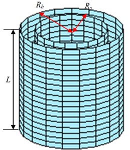
a) Holographic and reconstructed cylindrical surface

b) Holographic plane that has been discretized and expanded

5. Numerical simulations

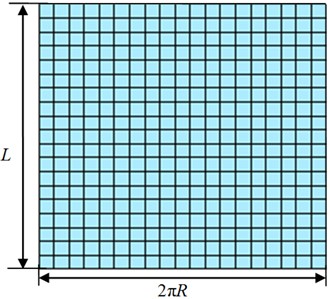
Numerical simulations have been firstly undertaken in this section to prove that the SOPA-NAH method can efficiently identify the vibration sources. The simulation model is an underwater cylindrical shell structure made from steel plates, and the finite element modeling of the cylindrical shell has been shown in Fig. 2.

The length of the cylindrical shell $L_1=$2 m, the radius $R_s=$ 0.3 m, and the density $\rho =$ 7800 kg/m. The speed of sound in water $c=$1500 m/s. Vertical excitations were applied to three different positions in the cylindrical shell, and only the vertical excitation and response in this numerical simulation were considered. The frequency range of the excitation force was 20 Hz-2000 Hz. Here, the holographic surface was a cylindrical surface with $R_h=$0.35 m, $L=$ 3 m, and the axial and circumferential sampling interval were $\mathrm{\Delta }z=L/M=3/51$ and $\mathrm{\Delta }\theta =2\pi /N=2\pi /37$.

Fig. 2Finite element model of a cylindrical shell and load location

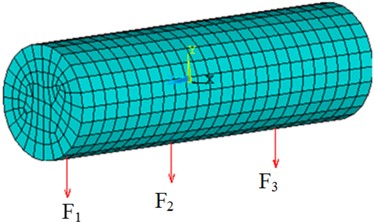
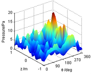
The cylindrical shell was modeled and its vibration response, due to the excitation force, was obtained by performing the finite element method (FEM) using ANSYS. The structural vibration response was used as a boundary condition for the shell boundary element model, and the underwater acoustic response was computed using the acoustic module of the Vibration Lab software. Then, the basic data, such as the response of the source points, the vibration response of the reference points and the holographic surface pressure, was obtained, which was used to perform the SOPA-NAH method. The excitation condition with $F_1=$2 N, $F_2=$2 N, $F_3=$0.6 N was selected, and a typical analysis frequency was 1707 Hz. The sound pressure distribution of the holographic surface has been shown in Fig. 3(a), which was expanded into the holographic plane as seen in Fig. 3(b). The reconstructed pressure distribution of the source surface can be obtained by solving Eq. (26) as shown in Fig. 4. It is obvious that the reconstructed sound field in Fig. 4(a) agreed well with the sound field in Fig. 4(b) computed by numerical simulation with only with slight differences in amplitude, thus verifying our cylindrical NAH technique.

Fig. 3Sound pressure distribution of the holographic surface at1707 Hz

a) Cylindrical surface

b) Expanding plane

In Fig. 4, the results of the sound pressure distribution and contribution cannot be determined from a single vibration source due to the cross-coupling between these sound sources. It will be difficult to accurately locate sound sources and efficiently implement vibration and noise control. To address this problem, the SOPA method was first applied to compute the sound field that radiated from each sound source. The selection of vibration source points and reference points is a significant topic when using the SOPA method. The selection of vibration source points should ensure that the points can reflect the characteristics of the vibration equipment and have a high signal to noise ratio. The selection of reference points should satisfy the requirement that the reference points are not identical to vibration effects and its vibration value should be the same order of magnitude. The number of sources was set as $m=$3, the number of reference points was set as $n1=2m=$6, the number of measurement blocks was set as $r=$4. Then, the SOPA-NAH method was performed with Eqs. (24)-(26) to identify the sound sources and predict the sound field.

The reconstructed sound field of each vibration source that was computed by the SOPA-NAH method has been illustrated in Figs. 5-7. These figures show that the reconstructed sound field in Figs. 5(a), 6(a), 7(a) is in good agreement with the sound field in Figs. 5(b), 6(b), 7(b) computed by numerical simulation, and the location of the sound sources and the amplitude of the pressure response can be accurately determined. There is a stronger cross-coupling from the vibration sources. This feature leads to the fact that the reconstruction result is a little larger than the calculation result. It is however believed that the computational accuracy is sufficient to meet the basic requirements of underwater noise analysis, as shown in Fig. 8. The calculation errors when the SOPA-NAH method was performed are derived from the discrete NAH formula and ignore the pressure contributions of the $x$-direction and $z$-direction.

Fig. 4Comparison of the reconstructed sound pressure and the numerical simulation of the cylindrical shell surface with all excitation forces run simultaneously at 1707 Hz

a) Reconstructed sound field distribution computed by the SOPA-NAH method

b) Sound field computed by numerical simulation

Fig. 5Comparison of the reconstructed sound pressure and numerical simulation of the cylindrical shell surface with #1 excitation force operating at 1707 Hz

a) Reconstructed sound field distribution computed by the SOPA-NAH method

b) Sound field computed by numerical simulation

Fig. 6Comparison of the reconstructed sound pressure and numerical simulation of the cylindrical shell surface with #2 excitation force operating at 1707 Hz

a) Reconstructed sound field distribution computed by the SOPA-NAH method

b) Sound field computed by numerical simulation

Fig. 7Comparison of the reconstructed sound pressure and numerical simulation of the cylindrical shell surface with #3 excitation force operating at 1707 Hz

a) Reconstructed sound field distribution computed by the SOPA-NAH method

b) Sound field computed by numerical simulation

Fig. 8Reconstruction error curve between the reconstructed sound pressure and the result of the numerical simulation

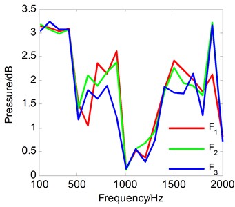
Fig. 9Total contribution curve of each vibration source to the measurement points of the cylindrical surface

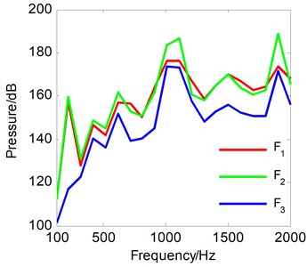
The SOPA-NAH method can identify and quantify the sound contribution of each vibration source to any sound field points, and the total contribution of each vibration source to the measurement points of the cylindrical surface has been shown in Fig. 9. It can be seen that the sound contribution of a vibration source may not be the same for different frequencies and even for the same frequency the contribution of each source may have similarities and differences. Fortunately, these can be analyzed qualitatively and quantitatively by the SOPA-HAN method. Fig. 9 has revealed that the contribution of the three vibration sources is #1>#2>#3 at 1707 Hz, #2>#1>#3 at 1010Hz, and #2>#1>#3 over the whole frequency range. We can also compute the contribution of various vibration sources for any point of the three-dimensional sound field by the SOPA-NAH method, which can overcome the blind, subjective and arbitrary analysis, and can ultimately obtain useful and reliable conclusions.

When the three excitation forces operate together, the reconstruction results for the typical frequency 1707 Hz based on the OPA-NAH and the SOPA-NAH method have been shown in Fig. 10, which agree well with the numerical simulation result shown in Fig. 4(b). As can be seen, the reconstruction error curves, as shown in Fig. 11, revealed that the errors between the reconstructed sound pressure and the numerical calculation value are generally less than 3 dB for the whole frequency range. This is mainly due to the fact that the measurement data are applied twice when performing the OPA technique, which always makes the OPA technique a better synthesis result. However, the OPA technique is more sensitive for other reference data, and it is also easy to get the wrong contribution. Therefore, the better synthesis result computed by the OPA technique, as shown in Fig. 10, cannot guarantee the effectiveness of the OPA technique. If we don’t understand the principle of the OPA technique, it is very easy to make mistakes in engineering judgment.

The vibration acceleration points which are close to the vibration equipment and have a larger vibration response are often selected as the input vibration sources for the OPA technique. This is feasible when weaker cross-coupling is assumed among the vibration sources. In practical situations however, stronger cross-coupling among sources usually exists i.e., the vibration energy can flow from one vibration source to another vibration source, which will make the traditional OPA technique fail. For example, after performing the traditional OPA technique depicted in Eq. (15), the sound pressure distribution of the cylindrical shell surface derived from the #3 vibration source can be obtained by Eq. (26), as shown in Fig. 12. From comparison with the numerical simulation result shown in Fig. 7(b), it can be seen that the reconstructed sound pressure became larger and the location of the maximum sound pressure distribution was inconsistent with the actual location due to the cross-coupling from #1 and #2 vibration sources. That is to say, the sound pressure distribution of the entire sound field was much larger than the actual measurement results, and the results cannot be trusted. But, in Fig. 7(a), it is obvious that the SOPA technique was better at avoiding cross-coupling among the vibration sources. Finally, it can be concluded that the SOPA-NAH method cannot only compute the sound field distribution of the cylindrical surface, but it can also reconstruct other 3-D sound field distributions, and moreover, it can locate a sound source and accurately predict the sound field.

Fig. 10Comparison of the reconstructed sound pressure cylindrical shell surface by different methods

a) OPA-NAH method

b) SOPA-NAH method

Fig. 11Reconstruction error curve between the reconstructed sound pressure with the OPA-NAH and SOPA-NAH method

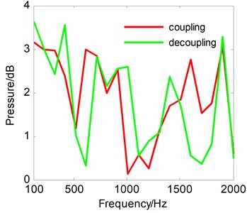
Fig. 12Sound pressure of the cylindrical shell surface reconstructed by the OPA-NAH method with the #3 excitation force operating at 1707 Hz

6. Experimental

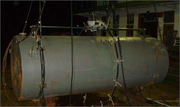
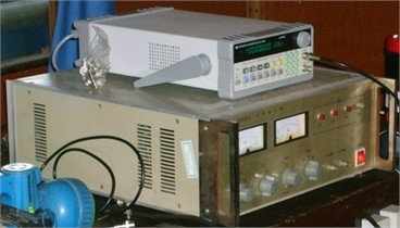
In an attempt to verify the feasibility and correctness of the SOPA-NAH method for sound source identification and field prediction, an experiment for measuring the underwater sound and vibration characteristics of the cylindrical shell model was carried out in open water. The length of the model was 1.8 m the radius was 0.51 m, and the model was placed 5 m underwater. The experimental model and measurement devices have been shown in Fig. 13. The holographic sound pressure was obtained using circular scanning equipment which was installed on the cabin model. The scanning radius was 0.71 m, the hydrophone line arrays had a 5^o interval, with 0.5 cm spacing in the axial direction. The reference hydrophones and accelerometers were arranged at the specific location inside or outside the cabin model. The measurement environment approximately met the free sound field conditions. There were two typical excitation sources i.e., an electromagnetic actuator and an electric pick actuator, which were placed in the cabin model and work at different excitation frequencies and energies. The sampling frequency was 20480 Hz, and the number of sampling points was 20480.

Fig. 13Experimental model and measurement equipment

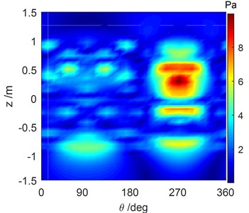
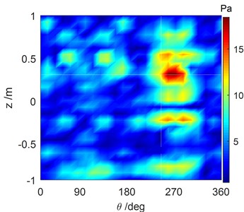
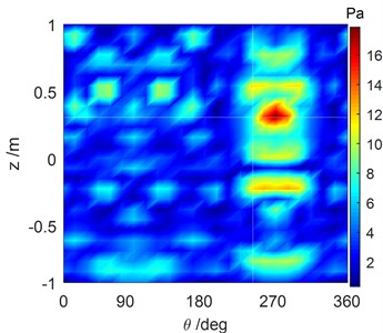
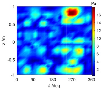
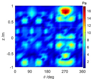
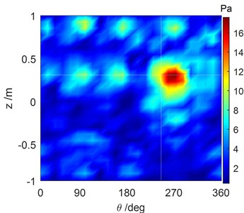
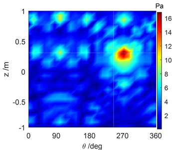
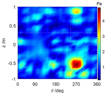
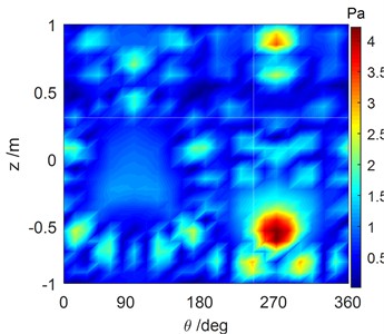
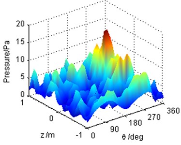
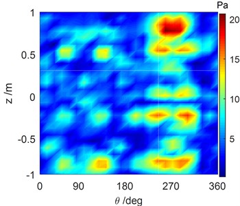
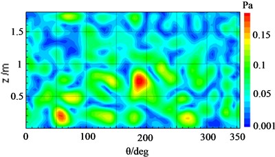
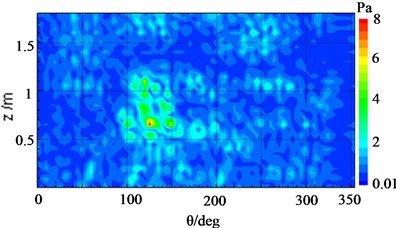
When both pieces of equipment ran simultaneously with excitation energy of 2Vpp, for a eigenfrequency of 920 Hz, Fig. 14(a) has shown that the reconstruction results of the cylindrical surface, which was computed by the cylindrical NAH technique, were in good agreement with the true pressure distribution depicted in Fig. 14(b). Nevertheless, it was difficult to distinguish the sound pressure distribution derived from a single vibration source due to the cross-coupling between the sound sources. In this case, the proposed SOPA-NAH method can be performed to address this issue. The reconstructed sound fields from each vibration source for each analyzed frequency have been shown in Fig. 15(a) for an electromagnetic actuator and Fig. 15(b) for an electric pick actuator, which agree well with the true sound field distribution seen in Fig. 16(a) and Fig. 16(b) respectively. It can also be seen that the SOPA-NAH method is superior to the traditional NAH technique which finds it difficult to analyze the impact of smaller sound sources on the entire sound field and accurately identify the location and size of the sound source. Therefore, it is clear that the proposed SOPA-NAH method can identify and quantify the main vibration source. Moreover, we can also determine the contribution of two vibration sources, i.e., the electromagnetic actuator has a larger influence than the electric pick actuator.

Fig. 14Sound pressure distribution of the holographic and reconstructed surface at 920 Hz

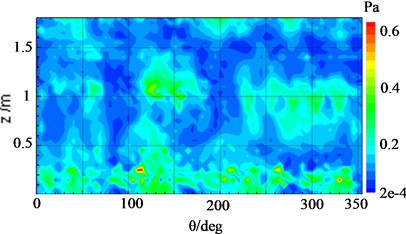
a) Holographic result

b) Reconstructed result

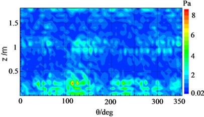
Fig. 15Comparison of the reconstructed sound pressure and true result of cylindrical shell surface with the electric pick actuator operating at 920 Hz

a) Reconstructed sound field distribution

b) The true result

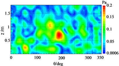
Fig. 16Comparison of the reconstructed sound pressure and the true result of the cylindrical shell surface with the electromagnetic actuator operating at 920 Hz

a) Reconstructed sound field distribution

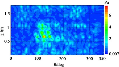
b) The true result

7. Conclusions

To identify and quantify the structure-borne sound source of a cylindrical shell effectively, the famous NAH and OPA techniques have been developed. Both techniques face a number of difficulties, which hardly lend them to be fit to practical requirements. The most important difficulty arises from the fact that the vibration sources usually pose stronger cross-coupling. Therefore, a new technique for separating coupling vibration sources has been proposed in this paper to address the aforementioned limitations. After overcoming the key issue in NAH and OPA techniques, and then combining the advantages of both techniques, a novel method named the SOPA-NAH method has been proposed for identifying the structure-borne sound source of the cylindrical shell. Firstly, numerical simulations were presented to prove the adaptability of the SOPA-NAH method. The results revealed that the reconstructed sound field of each vibration source agreed well with the sound field computed by numerical simulation with only slight differences in amplitude, verifying the SOPA-NAH technique. The proposed method is better at avoiding cross-coupling among the vibration sources which would lead to the reconstructed sound pressure becoming larger and the location of the maximum sound pressure distribution would be inconsistent with the actual location. The errors between the reconstructed sound pressure and the numerical calculation value were generally less than 3 dB for the whole frequency range. Therefore, the errors were still acceptable for sound source identification in practice. It is also possible to compute the contribution of various vibration sources for any points of the three-dimensional sound field by the SOPA-NAH method. Secondly, an experiment for measuring the underwater sound and vibration characteristics of a cylindrical shell model was carried out. It can also be concluded that the proposed SOPA-NAH method can identify and quantify the main vibration source, and moreover, can also determine the contribution of two vibration sources, i.e., the electromagnetic actuator has a larger influence than the electric pick actuator. That is to say, the SOPA-NAH method cannot only compute the sound field distribution of a cylindrical surface, but also reconstruct other 3-D sound field distributions, and moreover, it can locate a sound source and accurately predict the sound field.