Abstract
Road grade is important for autonomous vehicles, but it is difficult to measure directly. To address this issue, a hierarchical estimation of road grade is suggested based on the observation of tire forces. First, a 7-degree-of-freedom (DOF) dynamics model, including vehicle longitudinal, lateral, and yaw motions together with wheel rotations, is developed while considering the road grade. Subsequently, a dual-layer road grade estimation strategy is proposed based on an unscented Kalman filter (UKF). The lower-layer UKF estimates the longitudinal and lateral tire forces for road grade observation, and the upper-layer UKF is employed to estimate the road grade by considering the vehicle’s lateral acceleration and yaw rate. Finally, CarSim and MATLAB joint simulations and road tests are performed under different conditions to validate the correctness and effectiveness of the proposed estimation method. The results show that the proposed tire force observation-based estimator exhibits a lower mean absolute error and root mean square error on sloping roads and combined curved and sloping roads, and presents a better overall estimation performance on road grade compared with the widely used kinematics and dynamics model-based estimators.
Highlights
- A hierarchical estimation of road grade was proposed based on tire force observation.
- The lower-layer unscented Kalman filter (UKF) can accurately estimate the longitudinal and lateral tire forces; the upper-layer UKF presents a good estimation performance on the road grade.
- The proposed tire force observation-based estimator (TFOBE) presents high accuracy and robustness on grade estimation, and exhibits better performance than the usually used kinematics model-based estimator (KMBE) and driving equation-based estimator (DEBE) under different speed and road conditions.
1. Introduction
Road grade is a valuable external feedback signal during vehicle driving and can be used to build a three-dimensional map [1]. In addition, the road grade has an appreciable influence on the measurement of vehicle state properties, control strategy, and decision-making of automotive active safety control systems and driver assistance systems, such as the adaptive cruise control system and the autonomous emergency braking system [2]-[4]. Therefore, knowledge of road grade plays a vital role in enhancing the control accuracy of these systems.
Accurate direct measurement of road grades is challenging and expensive [2]. Consequently, vehicle kinematics or dynamics models are frequently used to estimate road grades. Kinematics model-based estimators (KMBEs) require longitudinal acceleration. However, the measured acceleration contains the vehicle acceleration and road grade information. Using a kinematics model to estimate the road grade requires decoupling the two signals. Kim et al. [5] suggested a vehicle kinematics model, and the road grade was estimated using a Kalman filter (KF), in which the vehicle longitudinal speed and longitudinal acceleration were described as the state variables, while the speed, acceleration, and gravity effects due to the road grade were described as the measurements. Hao et al. [6] identified road grade by steady-stable KF based on a kinematics model. Lin et al. [7] estimated the road grade using a KF considering vehicle acceleration and speed, coupled with the change rate of the road grade, which was identified in accordance with the derivatives of the measured and estimated accelerations. KMBE exhibits low accuracy when the vehicle rapidly accelerates or decelerates [8]. Therefore, Liu et al. [9] proposed an acceleration-adaptive interactive multiple-model algorithm to estimate road grade under smooth and intensive driving scenarios, and the vehicle pitch angle was adopted to enhance estimation accuracy under intensive driving conditions.
A dynamics model-based estimator can be established according to the vehicle longitudinal dynamics equation, also called the driving equation, in which the vehicle driving force equals the sum of the climbing resistance, rolling resistance, air resistance, and inertial resistance. This method commonly requires measurement of the engine torque, engine speed, vehicle speed, and transmission gear ratio. Vahidi et al. [8] suggested an estimator for vehicle mass and road grade based on recursive least squares (RLS) with forgetting factors. This method estimated the mass well but showed poor estimation of the road grade. Jo et al. [1] removed faulty measurements from a global positioning system (GPS) and vehicle onboard sensors using a probabilistic data association filter and then developed an interactive multiple-model filter to estimate the road grade. Lei et al. [11] and Liu et al. [12] decoupled road grade from vehicle mass using an extended Kalman filter (EKF). Su and Huang [13] proposed both the EKF and the unscented Kalman filter (UKF) to estimate road grade. The comparison results showed that the UKF had a higher accuracy than the EKF because the former needed to calculate the Jacobian matrix and inevitably introduced linearity errors. Ren et al. [14] addressed the time-varying system noise during road grade estimation by introducing a noise statistics estimator with forgetting factors based on the EKF. An adaptive EKF was utilized to update the state and measurement equations in real time to correct the noise statistics.
The driving equation-based estimator (DEBE), which requires the transmission gear ratio and lacks vehicle lateral responses, presents limitations under shifting, stopping, and cornering conditions [15]. Vehicle working conditions can be determined by vehicle speed, acceleration, and other signals. Under normal driving conditions, the UKF was employed by Qin et al. [15] to estimate the road grade, while short-range grade estimation was accomplished using a gated recurrent unit under special driving conditions, such as starting, shifting, braking, and stopping. Feng et al. [8] combined the kinematics and dynamics models to estimate road grade and suggested a probabilistic nearest-neighbor data association method to determine which model was most suitable under special conditions. Additionally, a dual KF (UKF) was proposed for each model. The lower-layer KF (UKF) was used to calculate the grade change rate, and the upper-layer KF (UKF) was used to estimate the road grade.
The aforementioned studies only focused on road grade estimation in straight-line driving conditions without considering the influences of vehicle lateral responses on the estimations. The vehicle lateral acceleration was adopted to correct the longitudinal acceleration in the longitudinal dynamics model in [16], where a combination of the interacting multiple model and a strong tracking filter was proposed to estimate the road grade. Furthermore, Gao et al. [17] corrected the vehicle longitudinal acceleration using the lateral acceleration and yaw rate and performed road grade estimation under complex conditions. However, lateral and yaw motions are not presented in these equations.
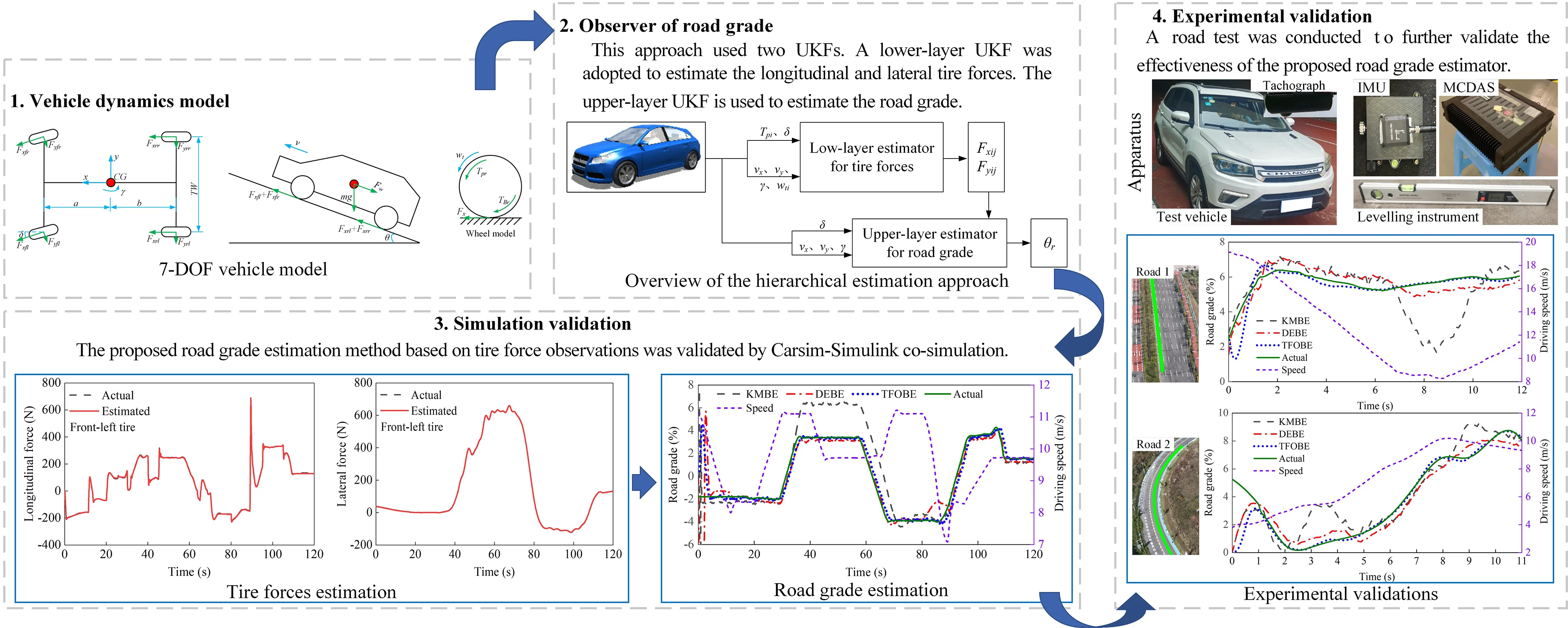
Longitudinal and lateral vehicle motions occur simultaneously during driving, particularly under cornering conditions. However, most traditional DEBEs [10]-[15] do not consider vehicle cornering responses, which results in a low tracking performance for estimators due to inaccurate vehicle models. In addition, these DEBEs replace the tire forces with the engine torque, neglecting the interaction forces between the vehicle wheels and road. Therefore, this study develops a 7-degree-of-freedom (DOF) vehicle model and presents a hierarchical estimator for road grade. The estimator is comprised of two layers. The longitudinal and lateral tire forces were estimated using a lower-layer UKF. The estimated forces were used as inputs for the upper-layer UKF, which was employed to estimate the road grade. Simulation and experimental validations demonstrated that the proposed estimator performed well in tracking road grade under different driving conditions. These findings can facilitate the further development of vehicle active safety control systems and driver assistance systems.
This study estimated the road grade under various speeds and road conditions using the simulation software MATLAB (r2019b Version) and CarSim (2020 Version). The undertaking method to enhance the structure and clarity is described in the following sections [18]:
Stage 1: Vehicle dynamics modeling with 7 DOFs.
Stage 2: Design of the hierarchical estimator, including a tire force observer and road grade observer.
Stage 3: Simulation and experimental validations.
2. Vehicle dynamics model
2.1. 7-DOF vehicle model
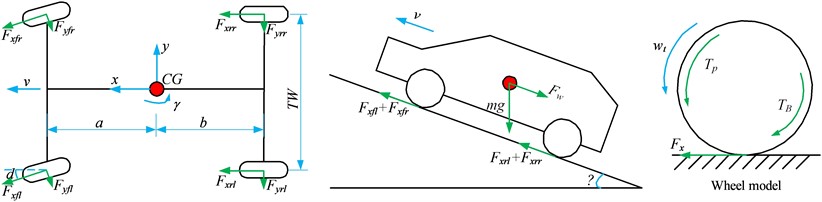
A 7-DOF vehicle model was established considering the road grade, as shown in Fig. 1. This model contains vehicle longitudinal, lateral, and yaw motions coupled with the rotations of the four wheels. The road bank, namely, the cross-slope, was assumed to be zero in this model.
Fig. 17-DOF vehicle model
According to D’Alembert’s principle, the longitudinal, lateral, and yaw motions of a vehicle are expressed as follows:
where is the vehicle mass; is the road grade; and denote the longitudinal and lateral velocity, respectively; is the yaw rate; represents the steering angle of front wheels; is the moment of inertia about the -axis of the vehicle; and are the distances from the vehicle mass center to the front and rear axles, respectively; is the track width; and denote the longitudinal and lateral tire forces, respectively; the subscript refers to , , and , representing the front-left, front-right, rear-left, and rear-right wheels, respectively; and is the acceleration of gravity. is the aerodynamic drag force and is described as follows:
where is the aerodynamic coefficient; and is the frontal area.
Rotational equations for the wheels are shown as:
where is the spin moment of inertia of the wheels; is the angular speed of the wheels; and refer to the driving torque and braking torque, respectively; and is the effective rolling radius of the wheels.
2.2. Tire model
The magic formula is typically used to describe tire forces. The longitudinal force for the pure longitudinal slip case and the lateral force for the pure lateral slip case are individually given as follows [19]:
where, , , , and are the factors of the longitudinal tire force; , , , and are the factors of the lateral tire force; and and denote the slip ratio and slip angle of the tires, respectively.
In addition, the slip ratio can be written as:
The slip angle can be given as:
Under a combination of braking and cornering conditions, the longitudinal and lateral forces of the tires are expressed as:
where:
The longitudinal and lateral tire forces are related to the vertical tire forces, which consist of the static load caused by the gravity of the vehicle and the dynamic load caused by accelerations:
2.3. Observer of road grade
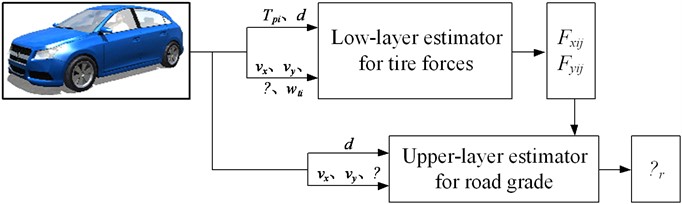
In this paper, a hierarchical estimation approach called the tire force observation-based estimator (TFOBE) is proposed. A basic overview of this estimation is shown in Fig. 2. This approach used two UKFs. A lower-layer UKF was adopted to estimate the longitudinal and lateral tire forces based on the 7-DOF model, in which the road grade was assumed to be zero. Here, the driving torque or braking torque of the wheels and steering angle are the inputs, and the vehicle speed, lateral acceleration, yaw rate, and wheel speed are the measurements. The upper-layer UKF is used to estimate the road grade based on a 3-DOF model as presented in Eqs. (1) to (3), by taking the estimated tire forces and steering angle as inputs and the vehicle speed, lateral acceleration, and yaw rate as measurements.
Fig. 2Overview of the hierarchical estimation approach
2.4. UKF
The vehicle model exhibited strong nonlinear characteristics, and the UKF algorithm is particularly suitable for solving nonlinear problems. The UKF algorithm was designed based on the Kalman linear framework. For the one-step prediction equation, an Unscented Transform was used to process the nonlinear propagation of the mean and covariance. The UKF algorithm is described as follows [8],[20]-[21]:
1. Initialization.
The state and the covariance of the state error are initialized here.
2. Time update.
Four steps were included: creating sigma points, predicting the state and its covariance, updating the sigma points, and predicting the measurements:
3. Measurement update
Two steps were included: calculating the KF gain, and updating the state and covariance:
3.1. Tire force observer
Tire forces play a critical role in influencing vehicle dynamics. The tire forces are typically divided into longitudinal, lateral, and vertical. Vertical tire forces are commonly calculated according to the vehicle mass and longitudinal and lateral accelerations [22],[23]. Thus, tire force acquisition mainly focuses on the longitudinal and lateral tire forces [23]. However, the tire forces are difficult to measure directly. Hence, estimation methods based on tire models are effective for obtaining the tire force [24]-[27].
The 7-DOF vehicle model was used to estimate the longitudinal and lateral tire forces. According to Eq. (12), when the road grade was 5 %, the vertical tire load changed by less than 2 % compared with a flat road. When the road grade was 10 %, the vertical tire load changed by approximately 4 %, and the longitudinal and lateral tire forces changed by approximately 4 %. Therefore, the road grade was not considered; that is, the road grade is equal to zero in Eq. (1) and Eq. (12) for the tire force observation. Similar simplification was practicable in [28]. The state and measurement equations for the lower-layer UKF observer are expressed as:
In this section, the state vector is defined as:
The measurement vector is:
The input is:
The state function is shown as:
where:
The state transition equations can be derived by discretizing the aforementioned system of equations, as shown in Eq. (30):
Here, is the sampling interval.
The measurement equation is:
Moreover:
The process noise covariance matrix = diag([1e-4; 1e-4; 8e-5; 1e-4; 1e-4; 1e-4; 1e-4; 1e-6; 1e-6; 1e-6; 1e-6; 1e-5; 1e-5; 1e-5; 1e-5]), and the measurement noise covariance matrix = diag([1e-4; 1e-4; 1e-4; 1e-4; 1e-4; 1e-4; 1e-4]).
3.2. Road grade observer
The longitudinal and lateral tire forces estimated by the lower-layer observer were used as inputs to the upper-layer observer, which was adopted to estimate the road grade. The rotational motion of the wheels was neglected in the estimation. Therefore, according to the 3-DOF model including the vehicle’s longitudinal, lateral, and yaw motions, as shown in Eqs. (1) to (3), the state vector of the upper-layer UKF observer is constructed as:
The measurement vector is:
The input is:
The state function is expressed as:
Moreover:
The measurement function is:
where:
The process noise covariance matrix = diag([1e-4; 1e-4; 1e-4; 1e-4]), and the measurement noise covariance matrix = diag([1e-2; 1e-2; 1e-2]).
4. Simulation validation
The proposed road grade estimation method based on tire force observations was validated by CarSim-Simulink co-simulation and compared with the typically adopted estimators [1], [5], [7], [8], [13], [15], namely KMBE and DEBE. KMBE and DEBE were realized using a KF and UKF, respectively.
The driving equation can be written as:
where, represents the torque from the engine or electric motor; and are the gear ratio of the transmission and the main reducer, respectively; is the mechanical efficiency of the powertrain; and is the friction coefficient.
The kinematics model can be expressed as:
where is the measured longitudinal acceleration.
The simulation data were output from the CarSim software, and the estimators were developed using MATLAB/Simulink. The road grade derived from CarSim was used as the actual value. The mean absolute error (MAE) and root mean square error (RMSE) were chosen as indicators to objectively evaluate estimation effectiveness. MAE and RMSE are defined as follows [8], [29]:
where and refer to the estimated road grade and actual grade at the -th moment, respectively.
4.1. Straight line and constant speed
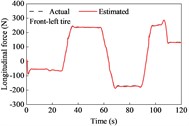
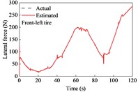
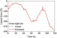
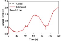
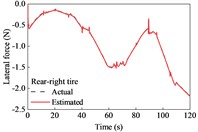
A straight and sloping road model was developed based on the elevation data of an interchange ramp in [30]. This road included four constant-grade sections and five transitional sections. The vehicle negotiated its drive on the road at a constant speed of 9.7 m/s. The estimation results for the longitudinal and lateral tire forces are shown in Fig. 3. The longitudinal forces were the driving forces for the upslope, and the maximum reached approximately 240 N. The longitudinal forces were the braking forces when moving on a downward slope, and the maximum was approximately 200 N. Because of the camber and toe angles, lateral tire forces exist for the left and right tires, even though the vehicle is driven straight. However, the sum of the lateral forces on the left and right tires was nearly 0 N. As shown in Fig. 3, the estimated tire forces are consistent with the actual values. This indicates that the longitudinal and lateral tire forces estimated using the UKF algorithm can effectively track the actual forces.
Fig. 3Tire forces estimation during straight-line and constant speed drive

The estimated tire forces were used as the input for the road grade estimator. The estimated road grade and errors are shown in Fig. 4 and Table 1. In the first 27 s, the vehicle negotiated a constant downgrade section of –1.8°; then it was driven on a transitionally sloping section for about 8.7 s where the road grade ranged from –1.8° to 3.5°; from 35.7 s to 57 s, it was driven on a constant upslope section of 3.4°, followed by a drive on a transitionally sloping section ranging from 3.4° to –3.9°; in the time range of 69-88 s, it negotiated a constant downgrade section of –3.9°, and this was followed by the drives on sloping sections and constant sections.
As shown in Fig. 4, the estimators show mismatches in the first several seconds, but the estimated road grades converge quickly and approach the actual grades. The proposed TFOBE and DEBE provide reliable conformity to the actual road grades, while the estimated values from KMBE appear to be lower than the actual values and exhibit large errors. When the road grade was constant, TFOBE exhibited a better estimation effect than DEBE. The estimation errors of TFOBE were slightly greater for transitional sections, but still exhibited high estimation accuracy. The MAE and RMSE of TFOBE were 0.133 % and 0.232 %, respectively, which were much lower than those of DEBE and KMBE. The estimated road grades in the first several seconds were not adopted in the calculation of the MAE and RMSE, as large jitters existed there. Similar processing methods were used in the following paragraph.
Fig. 4Road grade estimation results during straight-line and constant speed drive
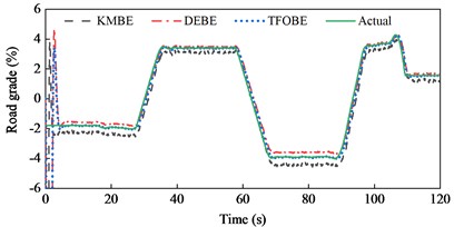
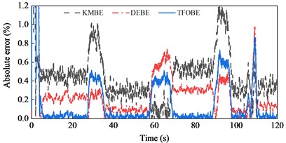
Table 1MAE and RMSE of road grade estimations during straight-line and constant speed drive
Project | KMBE | DEBE | TFOBE |
MAE | 0.437 % | 0.240 % | 0.133 % |
RMSE | 0.496 % | 0.291 % | 0.232 % |
4.2. Straight line and variable speed
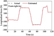
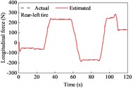
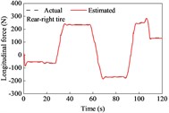
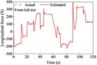
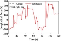
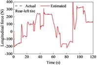
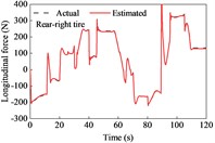
The vehicle was driven on straight and sloping roads at variable speeds. It underwent deceleration, acceleration, and variable-speed stages while negotiating on the road. The longitudinal tire forces were rather complex and changeable and showed a peak at approximately 90 s due of the variable-speed drive on the upslope and downgrade sections compared with the simulation at a constant speed, as shown in Fig. 5. However, the lateral forces exhibited similarities. The estimated tire forces were in good agreement with the actual forces.
Fig. 5Tire forces estimation during straight-line and variable-speed drive
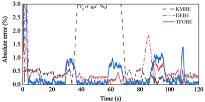
The road grade estimation results and absolute errors, along with the driving speed, are shown in Fig. 6. The estimation results from TFOBE and DEBE showed good agreement with the actual road grades. The absolute errors of the former estimator were smaller than those of the latter in the first 58 s, last 10 s, and between 68 and 70 s and 80 and 107 s. The maximum error of TFOBE was approximately 0.97 % at 109 s. DEBE showed a lower error in the simulation time range of 58-68 s, 70-80 s, and 107-110 s, but it did not match the actual grade from 81 s to 89 s. The maximum absolute error was 1.88 % at about 85.6 s when the driving speed and road grade both changed severely. KMBE exhibited larger estimation errors than the other estimators. In particular, abnormal peaks occurred when the driving acceleration changed, as observed at approximately 12.3 s, 21 s, and 46 s. The maximum absolute error was over 2 %.
The MAE and RMSE were calculated, as shown in Table 2. TFOBE provided the best estimation effect, followed by DEBE.
Fig. 6Road grade estimation results during straight-line and variable-speed drive
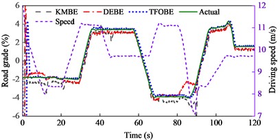
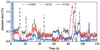
Table 2MAE and RMSE of road grade estimations during straight-line and variable-speed drive
Project | KMBE | DEBE | TFOBE |
MAE | 0.450 % | 0.352 % | 0.183 % |
RMSE | 0.612 % | 0.462 % | 0.250 % |
4.3. Cornering and variable speed
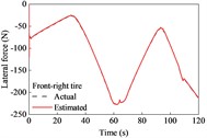
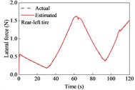
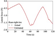
A combined curved and sloping road model was built based on the - coordinates and elevation data of the ramp. The vehicle was driven on the road at the aforementioned variable speeds. The estimated tire forces are shown in Fig. 7. The lateral forces of the front and rear tires were both larger than those when driving on a straight road. This is because relatively large lateral tire forces are required to act against the centrifugal force of the vehicle while driving along a curve. In this case, the tire force observer also provided good conformity with the actual observers.
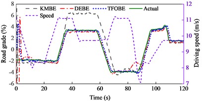
The estimated road grades, absolute errors, and driving speeds are shown in Fig. 8. The estimation results of TFOBE and DEBE are similar to those of the drive on a straight line. TFOBE exhibited a higher accuracy in the time range of 0-58 s, 69-89 s, 98-107 s, and the last 10 s, while the absolute errors of DEBE were lower within the other time sections. DEBE had large errors in the time range of 81–89 s, and the errors are also relatively noticeable from 5 to 12 s and from 21 to 29 s. The maximum estimated road grade of KMBE was over 6 %, and the error was approximately 3 % in the time range of 36-68 s, which was much larger than the actual value. This indicates that KMBE did not work well in this situation.
Table 3MAE and RMSE of road grade estimations during cornering and variable-speed drive
Project | KMBE | DEBE | TFOBE |
MAE | 1.09 % | 0.374 % | 0.271 % |
RMSE | 1.62 % | 0.488 % | 0.428 % |
The MAE and RMSE of TFOBE were 0.271 % and 0.428 %, respectively, which were much lower than those of the other estimators. This indicates that TFOBE exhibited the best performance for grade estimation. KMBE provided the worst estimation accuracy, with MAE and RMSE values of 1.09 % and 1.62 %, respectively.
Fig. 7Tire forces estimation during cornering and variable-speed drive
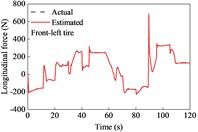
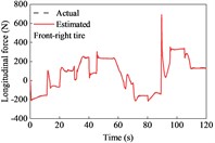


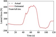
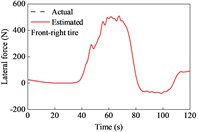
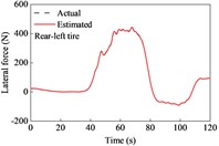

Fig. 8Road grade estimation results during cornering and variable-speed drive
5. Experimental validation
To further validate the effectiveness of the proposed road grade estimator, a road test was conducted on a rural road based on a real vehicle equipped with a multichannel data acquisition system (MCDAS), an inertial measurement unit (IMU), and a tachograph, as shown in Fig. 9.
Fig. 9Apparatus and test road
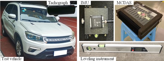
a) Apparatus
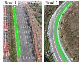
b) Test road
The MCDAS was used to collect real-time data from the Controller Area Network (CAN) Bus, including the engine speed, torque ratio percentage of the engine, vehicle speed, wheel speed, and braking pressure. The real-time engine torque can be calculated based on the maximum torque and torque ratio percentages. The IMU was used to measure the vehicle’s longitudinal velocity, longitudinal and lateral accelerations, and yaw rate. A tachograph was used to record the traffic environment and aid in data extraction from the demanded road section. In addition, a leveling instrument was used to measure the road grade.
The vehicle was driven on a rural road, on which two road sections were chosen to validate the proposed estimator. Road 1 was a straight upslope section with a length of about 140 m. Road 2 was a circular and upslope section and was about 100 m in extent.
The driving mission was accomplished continuously along the test route, and the vehicle driving data during the road test were collected by the MCDAS and IMU. The data obtained while negotiating Roads 1 and 2 were extracted based on the video image derived from the tachograph. Road grades were manually measured every several meters. Subsequently, the cubic spine interpolation fitting method was used to determine the actual grades of the road sections.
The estimation results for Road 1 are shown in Fig. 10. There is a slight jitter in the estimated curve derived from TFOBE within the first 2 s. However, the result quickly converges and presents a perfect estimation performance for the road grade, and the absolute error remained low after convergence. The estimation effects of DEBE and KMBE were worse than those of TFOBE overall; in particular, KMBE exhibited large errors in the time range of 7-10 s. The experimental validation for Road 2 is shown in Fig. 11. The results are similar to those for Road 1. Furthermore, the MAE and RMSE of TFOBE are much smaller than those of DEBE and KMBE for Roads 1 and 2, as shown in Table 4. This indicates that TFOBE is the most accurate and robust method.
Fig. 10Experimental validations of Road 1
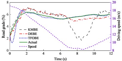
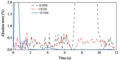
Fig. 11Experimental validations of Road 2
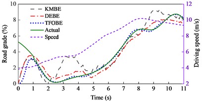
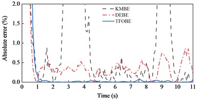
Table 4Experimental MAE and RMSE of road grade estimations
Road section | Project | KMBE | DEBE | TFOBE |
Road 1 | MAE | 1.14 % | 0.51 % | 0.09 % |
RMSE | 1.63 % | 0.53 % | 0.11 % | |
Road 2 | MAE | 0.88 % | 0.54 % | 0.10 % |
RMSE | 1.20 % | 0.58 % | 0.12 % |
6. Conclusions
In this study, a 7-DOF vehicle model was developed considering the road grade. Subsequently, a hierarchical estimator was designed to estimate road grade using a dual-layer UKF. The lower-layer UKF was used to observe the longitudinal and lateral tire forces. The upper-layer UKF was used to estimate the road grade. The performance of the proposed TFOBE was compared with that of commonly used methods, namely KMBE and DEBE. Simulation and experimental validation show that TFOBE performs well in estimating the road grade under different speeds and road conditions, and exhibits better accuracy and robustness than KMBE and DEBE. This indicates the validity and superiority of the hierarchical estimation approach based on the observation of tire forces.
An additional force exists along the lateral direction of the vehicle while cornering on a sloping road, which is equal to the vehicle weight multiplied by the product of the sine of the road grade and the sine of the vehicle heading angle [31]. The heading angle is the angle between the vehicle’s longitudinal direction and the road centerline, as presented in the literature [31], in which the normal tire forces were estimated based on the 3-DOF vehicle model (longitudinal, lateral, and yaw), considering the road grade angle. In this study, we hypothesized that the vehicle is driven along or parallel to the road centerline. Thus, the angle between the vehicle’s longitudinal direction and road centerline is rather small and can be ignored. In addition, the road grade is defined as the gradient of the road centerline and is less than 10 % [11], [17]. Therefore, the additional force is not presented in Eq. (2).
The proposed hierarchical estimator uses the UKF to estimate the road grade. Thus, the UKF was employed while conducting the estimation based on the driving equation, as presented in [8], [13], [15]. The 7-DOF model and driving equation were nonlinear, which was appropriate for the UKF. Nevertheless, the kinematics model is linear; thus, a KF is used to estimate the road grade based on this model [1], [5], [7]. Because the actual road grade at the beginning of the drive was not known, the initial road grade in the estimator was set to zero, which may have led to a large difference between the initial and actual values. Thus, the estimated road grade could not track the actual value in the first several seconds during simulation and experimental validations [14], [29]. Therefore, only the data estimated after convergence were used to calculate the MAE and RMSE [29].
The limitation of this work is that the estimation results of the longitudinal and lateral tire forces were not presented in the experimental validation because tire force transducers, such as Kistler RoaDyn [24], [25], are too expensive, and we could not afford to equip these sensors on a real test car. However, the tracking performance of the lower-layer observer on the tire forces was validated using CarSim and MATLAB joint simulations. Several studies have demonstrated the reliability and effectiveness of this approach, in which an EKF observer was constructed to estimate the lateral tire forces considering the lateral load transfer of the vehicle [26], and a UKF observer was proposed to estimate the longitudinal and lateral tire forces using a 3-DOF vehicle model with a random-walk tire force model [27]. Furthermore, this study aimed to estimate the road grade using a hierarchical estimation approach, and the estimation results were validated experimentally.
The way forward in this study includes the improvement of the real-time performance, accuracy, robustness of the road grade estimator, and the joint estimation of the road grade and road bank. In the future, we will conduct further research in these areas.
References
-
K. Jo, J. Kim, and M. Sunwoo, “Real-time road-slope estimation based on integration of onboard sensors with GPS using an IMMPDA filter,” IEEE Transactions on Intelligent Transportation Systems, Vol. 14, No. 4, pp. 1718–1732, Dec. 2013, https://doi.org/10.1109/tits.2013.2266438
-
E. Hashemi, R. Zarringhalam, A. Khajepour, W. Melek, A. Kasaiezadeh, and S.-K. Chen, “Real-time estimation of the road bank and grade angles with unknown input observers,” Vehicle System Dynamics, Vol. 55, No. 5, pp. 648–667, May 2017, https://doi.org/10.1080/00423114.2016.1275706
-
J. Marzbanrad and I. Tahbaz-Zadeh Moghaddam, “Self-tuning control algorithm design for vehicle adaptive cruise control system through real-time estimation of vehicle parameters and road grade,” Vehicle System Dynamics, Vol. 54, No. 9, pp. 1291–1316, Jun. 2016, https://doi.org/10.1080/00423114.2016.1199886
-
I. T.-Z. Moghaddam, M. Ayati, and A. Taghavipour, “Cooperative adaptive cruise control system for electric vehicles through a predictive deep reinforcement learning approach,” Proceedings of the Institution of Mechanical Engineers, Part D: Journal of Automobile Engineering, Vol. 238, No. 7, pp. 1751–1773, Mar. 2023, https://doi.org/10.1177/09544070231160304
-
S. Kim, K. Shin, C. Yoo, and K. Huh, “Development of algorithms for commercial vehicle mass and road grade estimation,” International Journal of Automotive Technology, Vol. 18, No. 6, pp. 1077–1083, Aug. 2017, https://doi.org/10.1007/s12239-017-0105-6
-
S. Hao, P. Luo, and J. Xi, “Estimation of vehicle mass and road slope based on steady-state Kalman filtering,” (in Chinese), Automotive Engineering, Vol. 40, No. 9, pp. 1062–1067, 2018, https://doi.org/10.19562/j.chinasae.qcgc.2018.09.009
-
N. Lin, S. Shi, L. Ma, and H. Wei, “Road grade estimation with grade change rate information,” (in Chinese), Journal of Jilin University (Engineering and Technology Edition), Vol. 46, No. 6, pp. 1845–1850, 2016, https://doi.org/10.13229/j.cnki.jdxbgxb201606012
-
J. Feng, D. Qin, Y. Liu, and X. Wang, “Real time estimation of road slope based on Dual Kalman filter and probabilistic nearest neighbor data association,” (in Chinese), Journal of Mechanical Engineering, Vol. 58, No. 16, p. 258, Jan. 2022, https://doi.org/10.3901/jme.2022.16.258
-
Y. Liu, L. Wei, Z. Fan, X. Wang, and L. Li, “Road slope estimation based on acceleration adaptive interactive multiple model algorithm for commercial vehicles,” Mechanical Systems and Signal Processing, Vol. 184, p. 109733, Feb. 2023, https://doi.org/10.1016/j.ymssp.2022.109733
-
A. Vahidi, A. Stefanopoulou, and H. Peng, “Recursive least squares with forgetting for online estimation of vehicle mass and road grade: theory and experiments,” Vehicle System Dynamics, Vol. 43, No. 1, pp. 31–55, Jan. 2005, https://doi.org/10.1080/00423110412331290446
-
Y. Lei, Y. Fu, K. Liu, H. Zeng, and Y. Zhang, “Vehicle mass and road grade estimation based on extended Kalman filter,” (in Chinese), Transactions of the Chinese Society for Agricultural Machinery, Vol. 45, No. 11, pp. 9–13, 2014, https://doi.org/10.6041/j.issn.1000-1298.2014.11.002
-
Z. Liu, S. Cheng, J. Liu, Q. Wu, L. Li, and H. Liang, “A novel braking control strategy for hybrid electric buses based on vehicle mass and road slope estimation,” Chinese Journal of Mechanical Engineering, Vol. 35, No. 1, p. 150, Dec. 2022, https://doi.org/10.1186/s10033-022-00823-z
-
Q. Su and P. Huang, “Comparative analysis on vehicle mass and road slope with the Kalman filter approach,” (in Chinese), Journal of Machine Design, Vol. 38, No. 7, pp. 105–109, 2021, https://doi.org/10.13841/j.cnki.jxsj.2021.07.018
-
Z. Ren, L. Shen, W. Huang, and X. Liu, “Real time estimation of vehicle quality and road slope based on adaptive extended Kalman filter,” (in Chinese), Journal of Vibration, Measurement and Diagnosis, Vol. 40, No. 4, pp. 758–764, 2020, https://doi.org/10.16450/j.cnki.issn.1004-6801.2020.04.019
-
D. Qin, K. Wang, J. Feng, Y. Liu, K. Cheng, and Y. Xia, “Road slope estimation based on unscented Kalman filtering and gated recurrent unit,” (in Chinese), Automotive Engineering, Vol. 41, No. 10, pp. 1547–1555, 2022, https://doi.org/10.19562/j.chinasae.qcgc.2022.10.009
-
H. Guo, L. Wang, X. Zhao, and Q. Dai, “Joint estimation of vehicle mass and road slope considering lateral motion,” (in Chinese), Journal of Jilin University (Engineering and Technology Edition), pp. 1–12, 2023, https://doi.org/10.13229/j.cnki.jdxbgxb20221061
-
L. Gao, Q. Wu, and Y. He, “Joint estimation of freight vehicle mass and road slope under complex conditions,” (in Chinese), Journal of Mechanical Engineering, pp. 1–16, 2023.
-
M. A. Mat Norman, M. R. Mohd Razean, M. H. Mohd Rosaidi, M. S. Ismail, and J. Mahmud, “Effect of fibre volume on the natural frequencies of laminated composite plate,” Materials Today: Proceedings, Vol. 75, pp. 133–139, Jan. 2023, https://doi.org/10.1016/j.matpr.2022.10.245
-
H. B. Pacejka and E. Bakker, “The magic formula tyre model,” Vehicle System Dynamics, Vol. 21, No. sup001, pp. 1–18, Jan. 1992, https://doi.org/10.1080/00423119208969994
-
Y. Liu, D. Cui, and W. Peng, “Vehicle state and parameter estimation based on adaptive anti-outlier unscented Kalman filter and GA-BPNN method,” Journal of Vibroengineering, Vol. 26, No. 1, pp. 139–151, Feb. 2024, https://doi.org/10.21595/jve.2023.23441
-
P. Yu, S. Tan, J. Guo, and Y. Song, “Data-driven optimal controller design for sub-satellite deployment of tethered satellite system,” Electronic Research Archive, Vol. 32, No. 1, pp. 505–522, Jan. 2024, https://doi.org/10.3934/era.2024025
-
H. Guo, H. Chen, D. Cao, and W. Jin, “Design of a reduced‐order non‐linear observer for vehicle velocities estimation,” IET Control Theory and Applications, Vol. 7, No. 17, pp. 2056–2068, Nov. 2013, https://doi.org/10.1049/iet-cta.2013.0276
-
H. Guo, Z. Yin, D. Cao, H. Chen, and C. Lv, “A review of estimation for vehicle tire-road interactions toward automated driving,” IEEE Transactions on Systems, Man, and Cybernetics: Systems, Vol. 49, No. 1, pp. 14–30, Jan. 2019, https://doi.org/10.1109/tsmc.2018.2819500
-
S. Cheng, C.-F. Li, X. Chen, L. Li, X.-H. Wu, and Z.-X. Fan, “A hierarchical estimation scheme of tire-force based on random-walk SCKF for vehicle dynamics control,” Journal of the Franklin Institute, Vol. 357, No. 18, pp. 13964–13985, Dec. 2020, https://doi.org/10.1016/j.jfranklin.2020.10.030
-
R. A. Cordeiro, A. C. Victorino, J. R. Azinheira, P. A. V. Ferreira, E. C. de Paiva, and S. S. Bueno, “Estimation of vertical, lateral, and longitudinal tire forces in four-wheel vehicles using a delayed interconnected cascade-observer structure,” IEEE/ASME Transactions on Mechatronics, Vol. 24, No. 2, pp. 561–571, Apr. 2019, https://doi.org/10.1109/tmech.2019.2899261
-
R. A. Cordeiro et al., “Road grades and tire forces estimation using two-stage extended Kalman filter in a delayed interconnected cascade structure,” in 2017 IEEE Intelligent Vehicles Symposium (IV), pp. 115–120, Jun. 2017, https://doi.org/10.1109/ivs.2017.7995707
-
C. Jing, H. Shu, Y. Song, and C. Guo, “Hierarchical control of yaw stability and energy efficiency for distributed drive electric vehicles,” International Journal of Automotive Technology, Vol. 22, No. 5, pp. 1169–1188, Jul. 2021, https://doi.org/10.1007/s12239-021-0104-5
-
H. Hamann, J. K. Hedrick, S. Rhode, and F. Gauterin, “Tire force estimation for a passenger vehicle with the Unscented Kalman Filter,” in 2014 IEEE Intelligent Vehicles Symposium (IV), pp. 814–819, Jun. 2014, https://doi.org/10.1109/ivs.2014.6856391
-
X. Li, J. Ma, X. Zhao, and L. Wang, “Intelligent two-step estimation approach for vehicle mass and road grade,” IEEE Access, Vol. 8, pp. 218853–218862, Jan. 2020, https://doi.org/10.1109/access.2020.3042656
-
S. Luo, G. Chen, and J. Xu, “Driving safety of articulated vehicle on a typical interchange,” International Journal of Vehicle Safety, Vol. 12, No. 3/4, p. 307, Jan. 2022, https://doi.org/10.1504/ijvs.2022.129626
-
Z. Ma, Y. Zhang, and J. Yang, “Velocity and normal tyre force estimation for heavy trucks based on vehicle dynamic simulation considering the road slope angle,” Vehicle System Dynamics, Vol. 54, No. 2, pp. 137–167, Dec. 2015, https://doi.org/10.1080/00423114.2015.1122817
About this article

This research was supported by the “National Natural Science Foundation Project of China”, grant number 52302431, the “Natural Science Foundation Project of Chongqing in China”, grant number cstc2021jcyj-msxmX0794, the “Joint Training Base Construction Project for Graduate Students in Chongqing”, grant number JDLHPYJD2021006, the “Research and Innovation Program for Graduate Students in Chongqing Jiaotong University”, grant number 2024S0068.
The datasets generated during and/or analyzed during the current study are available from the corresponding author on reasonable request.
Shuang Luo: conceptualization, methodology, validation, investigation, resources, data curation, writing-original draft preparation, writing-review and editing, supervision, funding acquisition. Zixin Huang: investigation, writing-original draft preparation, writing-review and editing. Guiyuan Chen: validation, investigation, writing-original draft preparation. Shuqun Yang: validation.
The authors declare that they have no conflict of interest.
