Abstract
Gears and bearings play vital roles as essential transmission components in mechanical drivetrains. Accurately predicting the remaining useful life (RUL) of these components is paramount to ensure optimal performance and prevent unexpected failures. To enhance the precision of RUL prediction, a novel method has been developed which involves constructing health indicators (HI) and implementing an adaptive dynamic weighting (ADW) on a gated dual attention unit (GDAU). The process commences by extracting multi-dimensional time-frequency domain features from vibration signals, which are then refined using an improved kernel principal component analysis (Adaptive Kernel Principal Component Analysis – AKPCA) to extract key components. Subsequently, the constructed HI is fine-tuned through an optimization process utilizing the exponentially weighted moving average method. Finally, the ADW strategy dynamically adjusts the input weights of the HI, and the GDAU model is employed to predict the RUL of gears and bearings. Experiment and comparison results have validated the effectiveness and advantages of the proposed method.
Highlights
- The monotonicity and trend indicators are combined to construct a new evaluation index and construct an adaptive AKPCA algorithm. This improvement reduces human intervention and achieves adaptive HI construction.
- To dynamically adjust weights, this study proposes an adaptive dynamic weighting method that adjusts the weight of feature weighting based on the importance of HI adaptively, thereby improving the accuracy of prediction.
- This study investigated the predictive performance of the proposed method on full-life data and compared it with traditional and currently advanced methods, verifying its superiority.
1. Introduction
Gears and bearings are common components of mechanical equipment, and they are prone to malfunctions due to harsh working environments and load changes. Monitoring their health status and predicting RUL to ensure smooth mechanical operation is crucial [1, 2]. In recent years, the existing RUL prediction methods can be roughly divided into two types: model-based and data-driven approaches [3, 4]. Model-based methods have achieved significant advancements, yet they encounter persistent challenges. Primarily, the complexity of accurately defining a physical model to encapsulate the intricate RUL dynamics in nonlinear systems remains a formidable hurdle [5, 6]. Additionally, the accuracy prediction of prevalent particle filtering methods is hampered by the issue of particle degradation [7]. Compared to model-driven methods, data-driven techniques do not necessitate the construction of intricate physical models, making them widely adopted in various fields. With the rapid advancement of artificial intelligence, data-driven deep learning has emerged as a prominent research focus within the realm of prognostic health management (PHM) [8, 9]. This trending approach utilizes the power of neural networks and machine learning algorithms to process complex datasets, leading to enhanced predictive capabilities and improved decision-making in predictive maintenance applications. For example, Ding et al. [10] introduced a novel approach for predicting Remaining Useful Life (RUL) which integrates extended causal convolution with exponential models. The key of their methodology is the creation of health indicators (HI) which captures the degradation of performance and the identification of the first prediction time (FPT). Similarly, Nie et al. [11] presented a predictive model based on a convolutional neural network (CNN) which uses feature fusion techniques. By employing the PCA algorithm for feature selection to derive sensitive health indicators (HI), they developed a 1DCNN model to forecast the RUL of bearings. The extracted HI served as the foundation for both training the model and making accurate predictions. Li et al. [12] introduced a novel RUL prediction methodology that relies on one transfer multilevel shrinkage attention time convolutional network. This innovative approach addresses the challenge of uneven feature distribution by capturing and incorporating relevant information from different levels of the data effectively. By using the power of attention mechanisms, the model can focus on the most informative features adaptively, leading to enhanced prediction accuracy. However, in nonstationary cases, the construction of HI is the primary task of RUL prediction, and selecting an appropriate HI helps to describe degradation patterns accurately and improve prediction accuracy [13, 14]. To construct a monotonic HI, Li et al. [15] proposed a degraded feature fusion model combined with a generalized failure threshold determination method, thereby improving the prediction accuracy of the remaining life. Wang et al. [16] introduced a novel approach for bearing RUL prediction by utilizing a multi-feature fusion strategy with Health Indicator (HI) and a weighted time convolutional network (WTCN). Their method not only demonstrated high prediction accuracy but also incorporated a new loss function to further enhance performance. However, the above method is based on CNN, and its receptive field is limited by the size and number of convolutional kernels, so its ability to capture remote information is limited. In addition, CNN faces difficulties in extracting temporal information from temporal data, which limits its application in RUL. Therefore, more and more researchers are inclined towards methods based on recurrent neural networks (RNNs), which focus on mining temporal information in data to establish a mapping relationship between data and degradation trends. Yan et al. [17] introduced a cutting-edge gear Remaining Useful Life (RUL) prediction model that uses the innovative ordered neuron long short-term memory (ON-LSTM) network. Diverging from conventional LSTM architectures, this model integrates a tree structure within LSTM, exploiting the inter-neuron sequence information to bolster its predictive prowess. In a similar vein, Qin et al. [18] devised an original LSTM network enriched with both macro and micro attention mechanisms, augmenting its predictive capabilities. Their approach also harnessed the isometric mapping algorithm (ISOMAP) to construct the HI, which was pivotal in enabling precise RUL forecasts for gears. Zhou et al. [19] proposed a novel dual line gated recursive unit (DTGRU) aimed at improving its adaptive ability to complex degraded trajectories, fully utilizing the differences between input data and adjacent time step hidden states to extract non-stationary information and achieve high prediction accuracy. Ma et al. [20] proposed an optimal design for the cargo box of a dump truck based on structure lightweight, and the design effect on bearing life degradation is also discussed.
Currently, end-to-end RUL prediction methods have received widespread attention [21-23]. However, due to the large scale of RUL data and the presence of a large amount of “dirty” data (In other words, the collected data set contains data of various noises, errors, anomalies, or other interference factors), these methods require corresponding processing of the data, and therefore cannot truly achieve end-to-end prediction. In addition, these methods not only have low accuracy but also increase computational costs, which is unacceptable in practical engineering. Therefore, the RUL method based on HI construction is still the mainstream method, which does not rely on building fault models, but uses intelligent data mining methods to find the relationship between historical sensor data and RUL. Therefore, as long as there is sufficient data, RUL prediction can be achieved. However, in practical situations, obtaining a large amount of lifespan data is a difficult task. Therefore, to solve this problem, Pająk et al. [24] proposed a new data enhancement method, which solved the problem of poor-quality data or limited and incomplete data sets. Similarly, Wen et al. [25] also put forward unique views on the application of time series enhancement.
In this paper, the construction method of adaptive HI and the residual life prediction method based on adaptive dynamic weighting and gated dual attention unit are proposed. This method does not need data enhancement and is suitable for RUL prediction with limited samples and variable speed. The main contributions of this study are as follows: 1) In response to the problem of manually selecting kernel functions for the KPCA algorithm, this study combined monotonicity and trend indicators to construct a new evaluation index and constructed an adaptive AKPCA algorithm. This improvement reduces human intervention and achieves adaptive HI construction. 2) To dynamically adjust weights, this study proposes an adaptive dynamic weighting method that adjusts the weight of feature weighting based on the importance of HI adaptively, thereby improving the accuracy of prediction. 3) This study investigated the predictive performance of the proposed method on full-life data and compared it with traditional and currently advanced methods, verifying its superiority. The remains of the paper are organized as follows: Section 2 is the theoretical background. The flow chart of the proposed method and its details are given in Section 3. Section 4 is experimental verification and result analysis. Section 5 is the conclusion.
2. Method background
2.1. Adaptive kernel principal component analysis (AKPCA)
Due to the presence of nonlinear signals that arise during the operation of complex systems, the accuracy of RUL predictions using deep learning algorithms tends to be limited, resulting in significant challenges for achieving precise and reliable predictions. Therefore, reducing data dimensions and constructing a monotonic trend HI is an urgent problem to be solved [26].
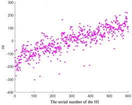
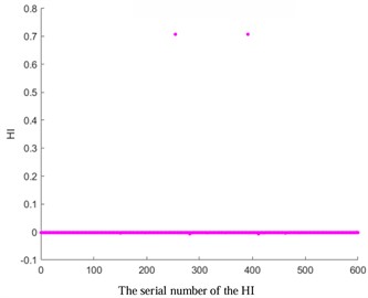
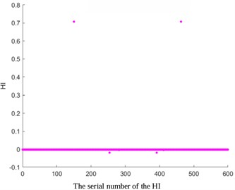
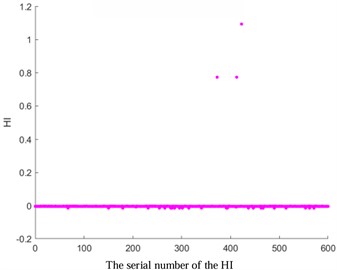
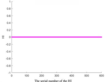
To enhance the efficiency of neural networks and streamline computational processes, the 21 time-domain and frequency-domain features were analyzed intricately and integrated into the RUL prediction model, as detailed in Table 1. In addition, to display the situation of extracting 21-dimensional features intuitively, the first six indicators in Table 1 are visually analyzed. As shown in Fig. 1, some features may not well represent the life degradation trend. Therefore, to improve the model performance and prediction accuracy, further extracting 21-dimensional features and fusing them are needed.
Fig. 1Feature visualization analysis: a)-f) correspond to the characteristics of indicators in Table 1
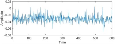
a) Peak to peak
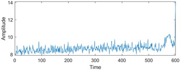
b) Peak
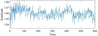
c) Mean
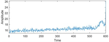
d) Variance
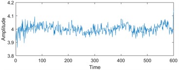
e) Root mean square
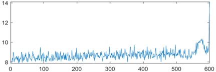
f) Absolute mean amplitude
By consolidating these multidimensional features into a new composite feature denoted as HI, the aim is to streamline computational complexity and enhance the overall predictive capability of the neural networks. In addition to neural networks, isometric mapping algorithms (ISOMAP) and kernel principal component analysis (KPCA) in manifold learning are commonly used methods for handling nonlinear data [27]. KPCA, as an extension of PCA, extracts principal elements from highly nonlinear features. By introducing a nonlinear kernel functionΦ, each sample xi of input data QN can be mapped to a high-dimensional feature F, and the covariance matrix in feature space F can be used to obtain the payload matrix. The payload Matrix refers to a set of feature vectors obtained by projecting the data in the original feature space into the kernel space. These eigenvectors describe the principal component direction and importance of data in the kernel space, which is equivalent to the representation of data after kernel transformation in the feature space. Finally, the covariance matrix in space F can be calculated as follows:
Table 121 calculation formulas for features
Index | Formula | Index | Formula |
Peak to peak | t1=Max|x(i)|-Min|x(i)| | Clearance factor | t10=Max|x(i)|(1N∑Ni|x(i)|1/2)2 |
Peak | t2=Max|x(i)| | Skewness factor | t11=1N∑Ni|x(i)|3(√1N∑Nix(i)2)3 |
Mean | t3=1N∑Nix(i) | Kurtosis factor | t12=1N∑Ni|x(i)|4(√1N∑Nix(i)2)4 |
Variance | t4=1N∑Ni(x(i)-ˉx)2 | Waveform factor | t13=√1N∑Nix(i)21N∑Ni|x(i)| |
Root mean square | t5=√1N∑Nix(i)2 | Mean frequency | f1=1N∑NjX(j) |
Absolute mean amplitude | t6=1N∑Ni|x(i)| | Frequency center | f2=∑Nj(f(j)*X(j))∑NjX(j) |
Impulsive factor | t7=Max|x(i)|1N∑Ni|x(i)| | Rms frequency | f3=√∑Nj(f(j)2*X(j))∑NjX(j) |
Standard deviation | t8=√1N∑Ni(x(i)-ˉx)2 | Standard deviation frequency | f4=√∑Nj((f(j)-fc)2*X(j))∑NjX(j) |
Peak factor | t9=Max|x(i)|√1N∑Nix(i)2 |
Among them, n is the quantity of input data. The loading matrix is the eigenvector of a covariance matrix C, represented as:
Among them, λ is the eigenvalue, and V is the eigenvector C of the covariance matrix. Given a set of vectors α=(α1,α2,⋯,αn)T, the description of the feature vector V is as follows:
By selecting the kernel function K(xi,xj), the kernel matrix K can be represented by K(Φ(xi),Φ(xj)). By combining Eqs. (1) and (3) above, the following could be concluded:
Then, Eigenvalue mλ and eigenvector K can then be computed, and the nonlinear mapping space F of Vk(k=1,2,⋯,n) for sample x in the final eigenvector is defined as:
Therefore, KPCA can determine whether the signal is normal with HotellingT2statistics. HotellingT2 can be calculated by the following formula:
Among them, ti(1×h) represents the principal component, P(n×h) represents the load matrix, Δ(h×h) represents the diagonal matrix formed, and Xi(1×n) represents the data in the i row of the 1×n-sample space. Hence, this innovative approach not only effectively retains the distinctive characteristics of the original data but also seamlessly uncovers intricate nonlinear connections inherent within these features.
However, the selection of kernel functions in the KPCA algorithm needs to be combined with specific data. To address this issue, we have made improvements. A new evaluation index was constructed by combining trends with monotonicity indicators. By integrating this evaluation indicator with KPCA, the kernel function can be selected based on the characteristics of the data adaptively. Among them, monotonicity can evaluate the trend property of a feature increasing or decreasing on the timeline. For feature sequence λ=[λ1,λ2,⋯,λn] and time series t=[t1,t2,⋯,tn], λt is the corresponding feature value at time t, and N is the maximum number of samples. The Trend calculation is as follows:
Among them, ¯λ is the average of {λi}i=1:N, and ¯T is the average of {ti}i=1:N. Furthermore, the calculation of monotonicity is as follows:
Among them, dλ refers to the differentiation of the feature sequence. Finally, a comprehensive evaluation index can be obtained, with a range of [0, 1]. The closer it is to 1, the better the construction of HI. The preset threshold is set within the comprehensive indicator range, where 0.8 is used to indicate that the feature sequence has good monotonicity. The calculation is as follows:
Based on common kernel functions: Gauss, Poly, Laplace, Linear, RBF, and Sigmoid. The test results of AKPCA are shown in Table 2, where 1 indicates a monotonic trend and 0 indicates no monotonic trend.
Table 2AKPCA experimental results
Type | Gauss | Poly | Laplace | Linear | RBF | Sigmoid |
Evaluation | 0 | 1 | 0 | 1 | 0 | 0 |
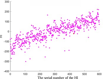
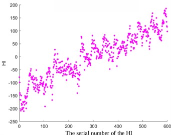
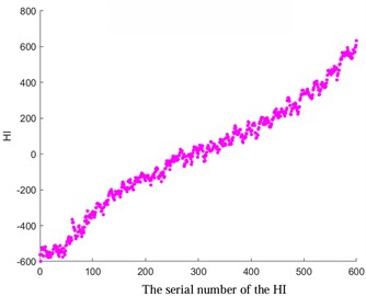
Fig. 2Comparative analysis of HI based on ISOMAP, KPCA Poly, and KPCA linear
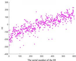
a) ISOMAP
b) KPCA-Poly
c) KPCA-Linear
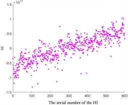
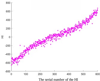
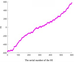
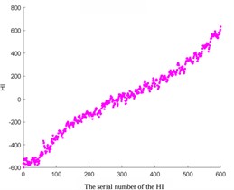
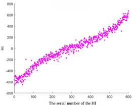
Fig. 3HI images of other kernel functions
a) KPCA-Laplace
b) KPCA-RBF
c) KPCA-Gauss
d) KPCA-Sigmoid
In addition, the ISOMAP algorithm and the KPCA algorithm based on Poly and Linear kernel functions were compared in Fig. 2. The results show that the trend of the ISOMAP algorithm is similar to that based on the KPCA algorithm. However, due to the high computational complexity of the ISOMAP algorithm, especially when dealing with large-scale data, it incurs significant computational time and space overhead. In addition, in the situation of data with noise and outliers, the algorithm can be affected, resulting in inaccurate results. In addition, compared to the KPCA algorithm, the ISOMAP algorithm is also more difficult to implement. Therefore, in the subsequent experiments, the KPCA algorithm based on the Linear kernel function was chosen considering the setting of prediction thresholds.
To verify the accuracy of AKPCA, HI images of other kernel functions as shown in Fig. 3 were displayed. The HI images based on Laplace, RBF, Gauss, and Sigmoid kernel functions do not exhibit a monotonic trend, which further proves the effectiveness of AKPCA.
2.2. Exponentially weighted moving average
In Fig. 2, it can be observed that the data shows a good degradation trend. Meanwhile, there is also a large degree of discreteness, which is unfavorable for subsequent RUL prediction. To solve this problem, the Exponentially weighted moving average was adopted to optimize the constructed HI. This algorithm considers the weight of historical data and assigns different weights to different historical data through exponential weighting. This algorithm not only reduces data noise and fluctuations effectively but also produces relatively smooth results. As shown in the following formula, by introducing a positive hyperparameter α∈(0,1), excessive smoothing is avoided and important health information is cleared:
Fig. 4Comparison before and after HI optimization
a) Original HI of pitting fault
b) HI optimized for pitting faults
c) The original HI of tooth breakage fault
d) Optimized HI for tooth breakage fault
Among them, xt and x't refer to the observed and estimated values at the time t. In this study, a specific value of 0.4 was selected (with lower values indicating greater smoothness). The results depicted in Fig. 4 demonstrate the favorable outcomes achieved through the implementation of the exponential weighted translation algorithm for optimization. Notably, HI showcases a consistent monotonic progression and enhanced smoothness, contributing significantly to the enhancement of predictive accuracy.
In addition, by comparing images with different smoothing factors (Fig. 5), it can be concluded that the smaller the smoothing factor, the higher the smoothness. Therefore, increasing the smoothing factor can avoid excessive smoothing and ensure that important details are not cleared.
Fig. 5Comparative analysis of different smoothing factors
a) The smoothing factor is 0.1
b) The smoothing factor is 0.4
c) Without treatment
2.3. Adaptive dynamic weighted gated dual attention unit
GRU successfully solves the problem of the disappearance of RNN gradient by introducing storage cells and related gate structures and can store information for a longer time [28, 29]. GRU is further improved based on LSTM, with a relatively simpler structure that only includes two gates: reset gate and update gate. Among them, the update gate integrates two gates of LSTM: input gate and forget gate, making GRU superior to LSTM in computation time and with less computational complexity. The reset gate can directly handle the previous hidden state. Some scholars have confirmed that through these two gating units, the GRU can control the output of information and determine which information can be output, thereby effectively preserving information from longer sequences and avoiding them from being cleared. The GRU architecture is shown in Fig. 6.
Fig. 6GRU structure
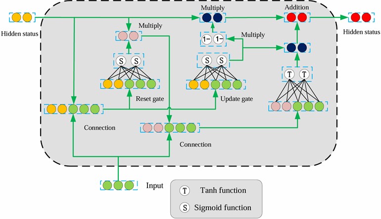
However, a single GRU is limited in its ability to make long-term predictions. Although GRU is designed to solve the problem of long-term dependence, due to the problem of gradient disappearance or gradient explosion in some cases, it is difficult to retain and transmit long-term memory, which affects its performance in long-term prediction tasks. Specifically, due to the problem of gradient propagation, GRU may suffer from long-term memory loss when processing long sequence data, which makes it difficult for the network to capture long-term dependencies in the sequence. Fortunately, the introduction of GDAU [30] has effectively addressed this issue. This innovative gate structure is designed to prioritize resetting and updating gate output information and includes an additional attention gate that focuses on input data as well as information from the previous hidden state. By incorporating two attention gates, the GRU model's capacity to address long-term dependency challenges is enhanced significantly. This not only reduces the required computational resources but also enables accurate predictions to be made even with limited sample data.
However, this network ignores the importance of adaptive dynamic weighting, so a self-adaptive dynamic weighting GDAU method is proposed based on GDAU architecture. We introduce a truncated normal distribution represented as ψ(ˉμ,ˉσ,a,b;x) in GDAU. Among them, ˉμ, ˉσ represents mean and variance. a, b represents the truncation interval. The probability density function is:
Its cumulative distribution function is:
Among them, ϕ(⋅), Φ(⋅) represent the probability density and distribution function of the standard normal distribution respectively. The inverse distribution of the cumulative distribution function: Let 0≤q≤1 find a≤x≤b so that:
From this, it can be inferred that:
It α=a-ˉμˉσ, β=b-ˉμˉσ is set, the mean is:
The variance is:
Therefore, by generating truncated normal distribution random numbers, random variables with specific means and standard deviations can be obtained. These random variables can be used as weights in the network to adjust the importance or influence of different inputs. Moreover, the dynamic adjustment of these weights allows the network to adapt flexibly to varying scenarios, taking into account the specific characteristics and distribution of the input data. This allows the model to allocate higher weights to critical features and time steps automatically, ultimately enhancing the accuracy and performance of Remaining Useful Life (RUL) predictions.
3. Prediction process
This study proposes an HI construction method and a gate-controlled dual attention unit prediction method based on adaptive dynamic weighting, achieving adaptive HI construction and remaining life prediction.
Fig. 7Prediction process
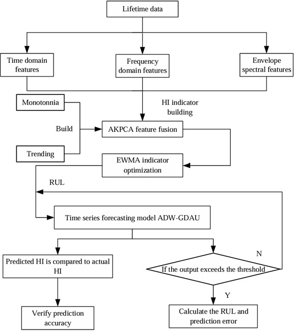
The model prediction process as illustrated in Fig. 7 consists of a series of specific steps that are crucial for accurately predicting RUL. These steps include:
1) Firstly, the 21-dimensional time-domain, frequency-domain, and envelope spectrum characteristics were calculated based on the full-life vibration samples collected from the experimental platform.
2) Secondly, a new evaluation index is constructed by combining monotonicity and trend indicators, and this evaluation index is integrated into KPCA to construct an adaptive AKPCA.
3) Then, the AKPCA algorithm is used to process these 21-dimensional high-dimensional features, and the constructed HI is optimized using the exponential weighted translation algorithm.
4) Subsequently, based on the constructed HI, further analysis of vibration sample data and feature data will be conducted to determine the required fault threshold for remaining life prediction.
5) Finally, the time series prediction model ADW-GDAU is used to predict the constructed HI to obtain the accurate RUL. Meanwhile, the information of prediction error is also obtained.
4. Case analysis
4.1. Data 1 description
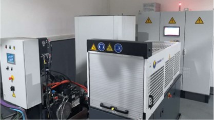
The dataset sourced from Chongqing University was utilized first. As depicted in Fig. 8, The testing machine is equipped with essential components such as a hydraulic cooling, torque control experimental operation system, and gear transmission platform. This study is divided into Remaining Useful Life (RUL) prediction under varied operating conditions, encompassing two distinct types of faults: tooth breakage and pitting corrosion. Considering that most of the data is in a stationary stage, we only used the last 600 samples to predict the RUL of the gears. Due to the good monotonic trend of the constructed HI, the last feature point of HI is selected as the fault threshold to terminate the prediction process.
Fig. 8Experimental platform
4.2. Parameter determination
The number of input units in the network plays an important role. In addition, learning rate is another key hyperparameter that can affect the training effectiveness and convergence speed of the model. Therefore, using grid search technology, these two hyperparameters are optimized by setting different input unit numbers and learning rates. Figs. 9 and 10 show the prediction error graphs, and the optimal parameters of the network were obtained based on them. Based on the prediction time in Table 3, it was determined that the number of neurons in the input layer, hidden layer, and output layer is set as 160, 22, and 1, respectively, along with employing an optimal learning rate of 0.05.
Fig. 9The impact of the number of input cells on RUL
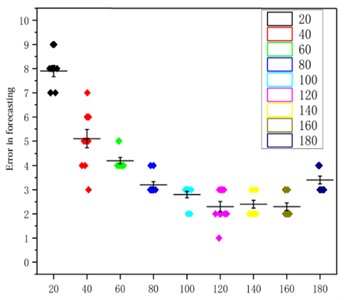
Fig. 10The impact of learning rate on RUL
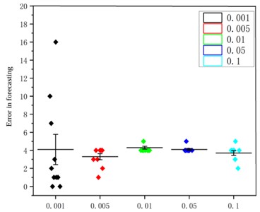
Table 3Effect of the number of input units on RUL prediction time
Input | 20 | 40 | 60 | 80 | 100 | 120 | 140 | 160 | 180 |
Time / s | 304 | 295 | 278 | 262 | 258 | 250 | 240 | 231 | 231 |
4.3. Experimental results and analysis
As depicted in Fig. 11, the prediction performance of the proposed RUL prediction method across varying RUL values is illustrated. It is evident that at RUL values of 25, 45, 65, and 85 minutes, the predicted RUL closely aligns with the actual RUL, displaying a consistent trend in the predicted values with the actual RUL values. The graph highlights that the proximity of the predicted point to the failure point correlates with the accuracy of gear RUL prediction, showing a higher accuracy. Furthermore, an increase in the number of known feature points leads to a significant enhancement of the network's predictive capability. When the number of feature points reaches 575, the accuracy of the predictions reaches an impressive 99 %. It is worth noting that 10 experiments were conducted on all subsequent methods to avoid unexpected errors, and their average values were recorded.
Fig. 11Comparison of different RUL prediction effects
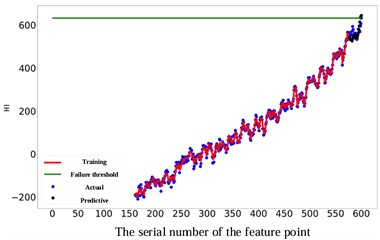
a) The actual RUL is 25
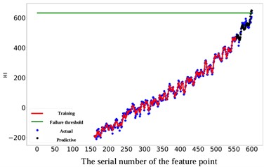
b) The actual RUL is 45
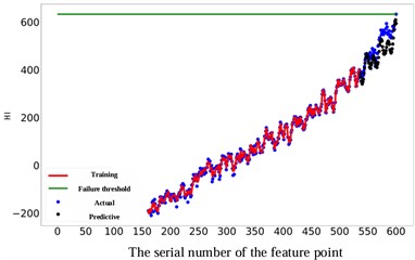
c) The actual RUL is 65
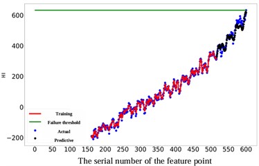
d) The actual RUL is 85
This study employs a scoring function (Score) and mean absolute error (MAE) as evaluation metrics for assessing the performance of the predictions. The Score metric imposes heavier penalties on late predictions, thereby providing a more comprehensive evaluation of the RUL prediction accuracy. The calculation of the score is specifically determined based on a detailed algorithm that considers various factors involved in the prediction process. The specific calculation of the score is as follows:
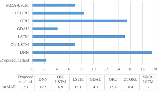
where, ActRul and GRul refer to actual Rul and predicted Rul. N indicates the number of experiments. The calculation of MAE is:
To verify the superiority of the proposed method, a comprehensive comparison was conducted with both traditional and advanced diagnostic models. By subjecting the proposed method to rigorous evaluation alongside established techniques, we aimed to highlight its effectiveness and innovative capabilities in the realm of predictive maintenance. Among them, the traditional methods include (1) DNN, (2) LSTM, (3) GRU; Advanced methods include (4) GDAU [30], (5) ON-LSTM [17], (6) MMA-LSTM [18], and (7) DTGRU [19]. From Figs. 12 and 13, it is evident that our method showcasing the highest scores and minimal errors consistently outperformed both traditional and advanced diagnostic models. This strongly suggests that our method offers superior accuracy in estimating the RUL. Furthermore, the comparison of life prediction results across various models clearly illustrates the significant enhancement in performance achieved by incorporating adaptive dynamic weighting modules into the GDAU model. The inclusion of these modules not only brings the life prediction results closer to actual values but also enhances the overall precision of life prediction, thereby solidifying the effectiveness and reliability of our approach.
Fig. 12Comparison of scores for various methods
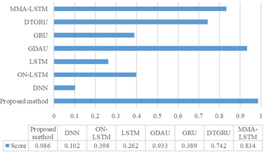
Fig. 13MAE comparison of various methods
To further prove the superiority of the model, we use the F1 score to evaluate the model. According to the results shown in Table 4, our method has achieved the best F1 score, which shows its excellent performance in model performance. Were, true positive (TP), false negative (FN), false positive (FP), true negative (TN). Therefore, the formula for calculating the F1- score is:
Table 4Comparison of F1 scores of each model
Proposed method | DNN | ON-LSTM | LSTM | GDAU | GRU | DTGRU | MMA-LSTM | |
F1-Scores | 0.980 | 0.333 | 0.837 | 0.571 | 0.913 | 0.529 | 0.783 | 0.837 |
To verify the performance of the proposed method under continuous prediction, we adjusted the number of input units (changed to 100) and the number of samples for continuous prediction (increased to 350). Fig. 14 shows the results of continuous prediction, indicating that continuous prediction can be achieved by changing the number of input units. In the figure, the predicted degradation trend is consistent with the actual degradation trend, which verifies the effectiveness of the method.
Fig. 14Effect of continuous prediction
Moreover, assessing the convergence speed of neural networks is crucial for evaluating their overall performance. In this context, the constructed Health Indicator (HI) was utilized to verify and analyze the convergence speed of the network. Fig. 15 shows the prediction error curve. It can be observed that after approximately 150 epochs, the network reached a stable state with minimal subsequent changes, which effectively proves the predictive stability of the model. In addition, to assess the generalization capability of the model, the RUL prediction was conducted on gears with pitting faults. The results illustrated in Fig. 16 highlight the continued strong performance of the proposed method in accurately predicting RUL for various types of faults. This outcome further corroborates the effectiveness and robustness of the model in handling different fault scenarios, underscoring its reliability and versatility.
4.4. Data 2 description
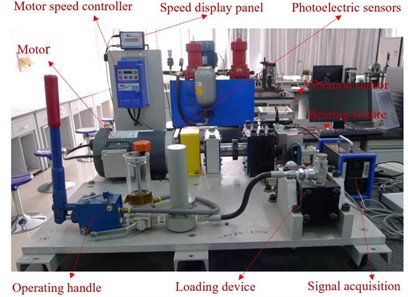
To verify the generalization of the model, a multifunctional bearing fault prediction experimental platform (BPS) developed by Spectra Quest was selected. We have developed our experimental platform as shown in Fig. 17 which comprises a radial loading device, speed display, vibration acceleration sensor, and data acquisition device. This setup was utilized to collect vibration data from the rolling bearings over their entire life cycle. This extensive testing and data collection strategy was implemented to validate and demonstrate the efficacy of the proposed method in predicting RUL. The bearing type is ERK16, and the experimental parameters are set as follows: a radial load of 8500 N is applied, with the speed fluctuating within the range of [1450-1550] r/min. Vibration data is sampled at a frequency of 12800 Hz, with a sampling interval of 5 minutes and a duration of each sampling period set at 4 seconds. These specific experimental conditions were carefully selected to ensure accurate and comprehensive data collection for the RUL prediction analysis of the rolling bearings.
Fig. 15Prediction error curve
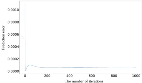
Fig. 16RUL of pitting failure
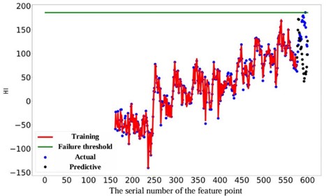
Fig. 17Test bench for predicting the lifespan of variable speed bearings
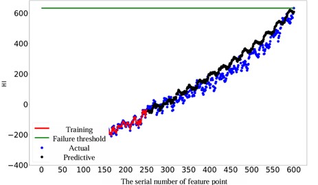
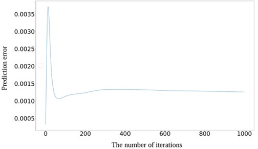
In this experiment, the neural network architecture was carefully designed with 50 neurons in the input layer, 17 neurons in the hidden layer, and 1 neuron in the output layer. A learning rate of 0.05 was determined to be optimal for the training process. The selection of these parameters aims to enhance the accuracy and reliability of the remaining life prediction analysis. We selected the last 300 samples for validation and determined the failure threshold based on the size of the last feature point. By utilizing the feature matrix composed of 285 experimental samples as the training dataset, predictions were generated for 15 different time points. The outcomes obtained via the suggested approach are illustrated in Table 5, where the AKPCA experimental results are detailed. Additionally, Fig. 18 showcases the training curve, prediction curve, and actual curve, providing a comprehensive visual representation of the analysis process and results. Based on the above curves, it is evident that the predicted curve closely follows the trend of the actual curve, suggesting that the proposed method forecasts the remaining lifespan of bearings under variable speed conditions effectively. Moreover, the average prediction error was found to be a mere 2.43 % through numerous experiments, showcasing the model’s robust generalization capability. The error curve depicting the prediction is illustrated in Fig. 19, revealing a gradual decrease and stabilization of prediction error with an increasing number of iterations. This observation serves to reinforce the efficacy of the proposed method, showcasing its consistency and reliability in predicting outcomes.
Table 5AKPCA experimental results
Type | Gauss | Poly | Laplace | Linear | RBF | Sigmoid |
Evaluation | 0 | 0 | 0 | 1 | 0 | 0 |
Fig. 18Failure thresholds, training, actual, and prediction curves for 300 experimental samples of real bearings
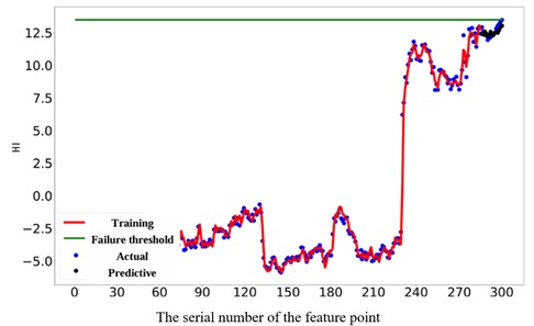
Fig. 19Prediction error curve
4.5. Discussion
Considering the environmental interference factors (including noise, electromagnetic interference, etc.) and the changes in speed and load, some features extracted may not well represent the life degradation trend in some cases. This emphasizes the importance of feature fusion because different feature sources can provide information from different aspects and angles. Through feature fusion, we can fuse this diverse information and get a more comprehensive and comprehensive feature representation to better reflect all aspects of data and the relationship between features. In addition, feature fusion also helps to reduce the sensitivity to noise or missing data, thus improving the stability and anti-interference ability of the model. Therefore, to improve the model performance and prediction accuracy, we adopt the strategy of extracting 21-dimensional features and fusing them. Such careful consideration and operation can effectively enhance the robustness of data features and provide more powerful support for further analysis and prediction. Moreover, judging from the results of the two case studies, we still achieved excellent prediction results even for complex working conditions and sudden changes. Besides, the invisible data can be reliably predicted.
5. Conclusions
A life prediction method is proposed in the article, which uses an improved neural network to fit the HI data of the constructed gears and bearings, and predicts their RUL through degradation curves. Due to the inability of a single feature to accurately determine the health status of gears and variable condition bearings, we have adopted multiple features. Specifically, we extracted 21-dimensional features from the time-domain, frequency-domain, and envelope spectra of gear and bearing vibration signals, and constructed a new HI through an improved KPCA algorithm and exponentially weighted moving average, thereby improving the accuracy of prediction. Furthermore, through enhancements made to the GDAU network, increased emphasis was placed on crucial features and timeframe intervals, enhancing the accuracy of the RUL prediction. The methodology puts forth demonstrated promising outcomes in two distinct case studies, showcasing its effectiveness and reliability.
It should be noted that in this article, the RUL threshold for health status was artificially set, which has a significant impact on experimental performance. In subsequent research, a unified threshold can be established to reduce human interference.
References
-
D. Chen, W. Cai, H. Yu, F. Wu, and Y. Qin, “A novel transfer gear life prediction method by the cross-condition health indicator and nested hierarchical binary-valued network,” Reliability Engineering and System Safety, Vol. 237, p. 109390, Sep. 2023, https://doi.org/10.1016/j.ress.2023.109390
-
Y. Qin, J. Yang, J. Zhou, H. Pu, X. Zhang, and Y. Mao, “Dynamic weighted federated remaining useful life prediction approach for rotating machinery,” Mechanical Systems and Signal Processing, Vol. 202, p. 110688, Nov. 2023, https://doi.org/10.1016/j.ymssp.2023.110688
-
Y. Ge et al., “Prediction of remaining life of rotating machinery based on t-SNE and LSTM,” (in Chinese), Vibration and Shock, Vol. 39, No. 7, pp. 223–231, 2020, https://doi.org/10.13465/j.cnki.jvs.2020.07.031
-
Q. S. Jiang et al., “Prediction method of remaining life of rolling bearings based on dynamic weighted convolutional long short-term memory network,” (in Chinese), Vibration and Shock, Vol. 41, No. 17, pp. 282–291, 2022, https://doi.org/10.13465/j.cnki.jvs.2022.17.035
-
H. Liang, J. Cao, and X. Zhao, “Multi-sensor data fusion and bidirectional-temporal attention convolutional network for remaining useful life prediction of rolling bearing,” Measurement Science and Technology, Vol. 34, No. 10, p. 105126, Oct. 2023, https://doi.org/10.1088/1361-6501/ace733
-
Y. Shang, X. Tang, G. Zhao, P. Jiang, and T. Ran Lin, “A remaining life prediction of rolling element bearings based on a bidirectional gate recurrent unit and convolution neural network,” Measurement, Vol. 202, p. 111893, Oct. 2022, https://doi.org/10.1016/j.measurement.2022.111893
-
W. Du, X. Hou, and H. Wang, “Time-varying degradation model for remaining useful life prediction of rolling bearings under variable rotational speed,” Applied Sciences, Vol. 12, No. 8, p. 4044, Apr. 2022, https://doi.org/10.3390/app12084044
-
H. L. Li et al., “A bearing life prediction method based on TC-CAE,” (in Chinese), Vibration and Shock, Vol. 41, No. 14, pp. 105–113, 2022, https://doi.org/10.13465/j.cnki.jvs.2022.14.015
-
J. Yan, Z. He, and S. He, “Multitask learning of health state assessment and remaining useful life prediction for sensor-equipped machines,” Reliability Engineering and System Safety, Vol. 234, p. 109141, Jun. 2023, https://doi.org/10.1016/j.ress.2023.109141
-
W. Ding, J. Li, W. Mao, Z. Meng, and Z. Shen, “Rolling bearing remaining useful life prediction based on dilated causal convolutional DenseNet and an exponential model,” Reliability Engineering and System Safety, Vol. 232, p. 109072, Apr. 2023, https://doi.org/10.1016/j.ress.2022.109072
-
L. Nie, L. Zhang, S. Xu, W. Cai, and H. Yang, “Remaining useful life prediction for rolling bearings based on similarity feature fusion and convolutional neural network,” Journal of the Brazilian Society of Mechanical Sciences and Engineering, Vol. 44, No. 8, Jul. 2022, https://doi.org/10.1007/s40430-022-03638-0
-
W. Li, Z. Shang, M. Gao, S. Qian, and Z. Feng, “Remaining useful life prediction based on transfer multi-stage shrinkage attention temporal convolutional network under variable working conditions,” Reliability Engineering and System Safety, Vol. 226, p. 108722, Oct. 2022, https://doi.org/10.1016/j.ress.2022.108722
-
Y. Pan, T. Wu, Y. Jing, Z. Han, and Y. Lei, “Remaining useful life prediction of lubrication oil by integrating multi-source knowledge and multi-indicator data,” Mechanical Systems and Signal Processing, Vol. 191, p. 110174, May 2023, https://doi.org/10.1016/j.ymssp.2023.110174
-
M. Pająk, “Fuzzy model of the operational potential consumption process of a complex technical system,” Facta Universitatis, Series: Mechanical Engineering, Vol. 18, No. 3, pp. 453–472, Oct. 2020, https://doi.org/10.22190/fume200306032p
-
X. Li, W. Teng, D. Peng, T. Ma, X. Wu, and Y. Liu, “Feature fusion model based health indicator construction and self-constraint state-space estimator for remaining useful life prediction of bearings in wind turbines,” Reliability Engineering and System Safety, Vol. 233, p. 109124, May 2023, https://doi.org/10.1016/j.ress.2023.109124
-
H. Wang, X. Zhang, X. Guo, T. Lin, and L. Song, “Remaining useful life prediction of bearings based on multiple-feature fusion health indicator and weighted temporal convolution network,” Measurement Science and Technology, Vol. 33, No. 10, p. 104003, Oct. 2022, https://doi.org/10.1088/1361-6501/ac77d9
-
H. Yan, Y. Qin, S. Xiang, Y. Wang, and H. Chen, “Long-term gear life prediction based on ordered neurons LSTM neural networks,” Measurement, Vol. 165, p. 108205, Dec. 2020, https://doi.org/10.1016/j.measurement.2020.108205
-
Y. Qin, S. Xiang, Y. Chai, and H. Chen, “Macroscopic-microscopic attention in LSTM networks based on fusion features for gear remaining life prediction,” IEEE Transactions on Industrial Electronics, Vol. 67, No. 12, pp. 10865–10875, Dec. 2020, https://doi.org/10.1109/tie.2019.2959492
-
J. Zhou, Y. Qin, J. Luo, S. Wang, and T. Zhu, “Dual-thread gated recurrent unit for gear remaining useful life prediction,” IEEE Transactions on Industrial Informatics, Vol. 19, No. 7, pp. 8307–8318, Jul. 2023, https://doi.org/10.1109/tii.2022.3217758
-
Z. Ma, C. Liu, and M. Li, “Optimal design of cargo-box of dump truck based on structure lightweight,” Machinery design and manufacture, No. 12, pp. 145–149, 2018, https://doi.org/en.cnki.com.cn/article_en/cjfdtotal-jsyz201812040.htm
-
H. Liu, Z. Liu, W. Jia, and X. Lin, “Remaining useful life prediction using a novel feature-attention-based end-to-end approach,” IEEE Transactions on Industrial Informatics, Vol. 17, No. 2, pp. 1197–1207, Feb. 2021, https://doi.org/10.1109/tii.2020.2983760
-
Q. Zhu, Q. Xiong, Z. Yang, and Y. Yu, “A novel feature-fusion-based end-to-end approach for remaining useful life prediction,” Journal of Intelligent Manufacturing, Vol. 34, No. 8, pp. 3495–3505, Sep. 2022, https://doi.org/10.1007/s10845-022-02015-x
-
X. Su, H. Liu, L. Tao, C. Lu, and M. Suo, “An end-to-end framework for remaining useful life prediction of rolling bearing based on feature pre-extraction mechanism and deep adaptive transformer model,” Computers and Industrial Engineering, Vol. 161, p. 107531, Nov. 2021, https://doi.org/10.1016/j.cie.2021.107531
-
M. Pająk, M. Kluczyk, Muślewski, D. Lisjak, and D. Kolar, “Ship diesel engine fault diagnosis using data science and machine learning,” Electronics, Vol. 12, No. 18, p. 3860, Sep. 2023, https://doi.org/10.3390/electronics12183860
-
Q. Wen, L. Sun, and X. Song, “Time series data augmentation for deep learning: a survey,” arXiv:2002.12478, 2020.
-
Y. Wang, J. Wang, S. Zhang, D. Xu, and J. Ge, “Remaining useful life prediction model for rolling bearings based on MFPE-MACNN,” Entropy, Vol. 24, No. 7, p. 905, Jun. 2022, https://doi.org/10.3390/e24070905
-
Y. Pan, R. Hong, J. Chen, J. Feng, and W. Wu, “Performance degradation assessment of wind turbine gearbox based on maximum mean discrepancy and multi-sensor transfer learning,” Structural Health Monitoring, Vol. 20, No. 1, pp. 118–138, Jun. 2020, https://doi.org/10.1177/1475921720919073
-
Z. Jiang, J. Che, M. He, and F. Yuan, “A CGRU multi-step wind speed forecasting model based on multi-label specific XGBoost feature selection and secondary decomposition,” Renewable Energy, Vol. 203, pp. 802–827, Feb. 2023, https://doi.org/10.1016/j.renene.2022.12.124
-
H. Wang, M.-J. Peng, A. Ayodeji, H. Xia, X.-K. Wang, and Z.-K. Li, “Advanced fault diagnosis method for nuclear power plant based on convolutional gated recurrent network and enhanced particle swarm optimization,” Annals of Nuclear Energy, Vol. 151, p. 107934, Feb. 2021, https://doi.org/10.1016/j.anucene.2020.107934
-
Y. Qin, D. Chen, S. Xiang, and C. Zhu, “Gated dual attention unit neural networks for remaining useful life prediction of rolling bearings,” IEEE Transactions on Industrial Informatics, Vol. 17, No. 9, pp. 6438–6447, Sep. 2021, https://doi.org/10.1109/tii.2020.2999442
About this article

The authors have not disclosed any funding.
The datasets generated during and/or analyzed during the current study are available from the corresponding author on reasonable request.
The authors declare that they have no conflict of interest.
