Cross domain fault diagnosis method based on MLP-mixer network

Mao, Xiaodong

doi:10.21595/jme.2023.23460

Journal of Measurements in Engineering

Browse Journal

Submit article

Published: 30 October 2023

Check for updates

Cross domain fault diagnosis method based on MLP-mixer network

Xiaodong Mao¹

¹Department of Electronic Information Engineering, Yongcheng Vocational College, Yongcheng, 476600, China

Cite the article Download PDF

Downloads 102

Abstract

The quality of rolling bearings determines the safety of mechanical equipment operation, and bearings with more precise structures are prone to damage due to excessive operation. Therefore, cross domain fault diagnosis of bearings has become a research hotspot. To better improve the accuracy of bearing cross domain fault diagnosis, this study proposes two models. One is a cross domain feature extraction model constructed using a mixed attention mechanism, which recognizes and extracts high-level features of bearing faults through channel attention and spatial attention mechanisms. The other is a bearing cross domain fault diagnosis model based on multi-layer perception mechanism. This model takes the feature signals collected by the attention mechanism model as input to identify and align the differences between the source and target domain features, facilitating cross domain transfer of features. The experimental results show that the mixed attention mechanism model has a maximum accuracy of 97.3 % for feature recognition of different faults, and can successfully recognize corresponding signal values. The multi-layer perception model can achieve the highest recognition accuracy of 99.5 % in bearing fault diagnosis, and it can reach a stable state when it iterates to 26, and the final stable loss value is 0.28. Therefore, the two models proposed in this study have good application value.

1. Introduction

Rolling bearings, as important components of mechanical equipment, have important application value in industrial production. They are widely used in various industrial and agricultural production occasions [1]. Due to the complex and ever-changing working environment, the occurrence rate of faults is relatively high, which can easily cause significant economic losses and personal injury accidents. Therefore, how to ensure the safe operation of rolling bearings is a research hotspot in mechanical manufacturing. The traditional fault diagnosis method uses neural network technology. Although this technology can process vibration signals and construct their time-frequency maps through continuous wavelet transform, the computational accuracy of this method is relatively low [2]. There are still problems with incomplete feature recognition and poor transferability of cross domain features in current bearing fault diagnosis. This study addresses two current fault diagnosis issues. Compared with other methods that emphasize more obvious high-level features, this study innovatively combines the hybrid attention mechanism (AM) to construct a bearing cross domain feature diagnosis (CDFD) model, which collects and extracts both high and low-level features through the channel and the spatial AMs, to achieve the ability to completely identify the fault feature signal [3]. However, the mixed AM model cannot effectively solve the decline of cross domain feature diversion, so this study uses the multi-layer perception machine (MLP-Mixer) algorithm to build a CDFD model for bearings on the basis of the AM model. This model takes the feature signals collected by the AM model as input values, and adds two feature correction modules during the operation to correct and balance the feature differences in different domains to achieve the effect of not losing information when features transfer across domains [4]. To complete the above research content, the article is divided into five parts. The first part is an overall overview of the research content. The second part provides a review of the current research status on bearing fault diagnosis. The third part is divided into two sections, which respectively study the application principles of AM and MLP-Mixer algorithm in bearing fault diagnosis. The fourth part analyzes the application performance of the above two algorithms. The fifth part is a summary of the research content and results of the entire article.

2. Related works

The safety of rolling bearings plays an important role in the operation of mechanical equipment. At present, bearing fault diagnosis has become a research hotspot, and many scholars have explored it. Liu et al. [5] developed an eddy current sensing film diagnostic method that used current detection of bearing thickness to determine the bearing damage. The experimental results indicated that this method was feasible. Tang et al. [6] proposed using discrete digital models for bearing fault diagnosis. First, the original current signal of the bearing was measured by the probability density function, and then the characteristics of the original current were extracted and recognized according to the distributed discrete digital model. The effectiveness of this algorithm has been demonstrated through simulation experiments. Wang et al. [7] constructed a bearing fault warning model using empirical mode decomposition algorithm. Firstly, the empirical mode decomposition algorithm was used to extract and process the signal, obtain the corresponding signal entropy, and then calculate the fault feature vector based on the signal entropy, ultimately achieving fault warning. The experimental results showed that the accuracy of early warning was above 94 %, and the alarm time was about 0.27 seconds. Yin et al. [8] proposed using a combination of materials with high elastic modulus to optimize the bearing structure to reduce the causes of bearing friction failures. Through the screening of wear and friction experiments, the results showed that the bearing using the combination of YN6X/SiC material had the optimal friction performance. Cui et al. [9] conducted research on bearing faults in wind turbines. Firstly, a three-stage learning algorithm was constructed by combining fault feature vectors and regression functions. Then, sensitivity analysis was performed on fault features based on this algorithm to extract advanced features. The experimental results indicated that this algorithm had certain application value in the wind turbine fault diagnosis. Zhang et al. [10] proposed to optimize the deep learning fault diagnosis model to address the poor alignment of edge features in bearing fault diagnosis. The optimization model introduced adversarial learning to extract edge features and used a weighting mechanism to reflect them. The experimental results indicated that the optimization model could effectively solve the CDFD. Chen et al. [11] proposed a fault diagnosis regression framework to solve fault diagnosis in complex scenarios. This framework used adversarial domain invariant generalization to diagnose fault features, while feature normalization and adaptive weight methods were also used to improve diagnostic performance. The experimental results indicated that this framework could be effectively applied to CDFD of bearings in complex scenarios. Wang et al. [12] constructed a new type of fault diagnosis model using SATLN network to improve the accuracy of fault diagnosis. This model extracted transferable features of faults through convolution operations, and then constructed corresponding target subdomains to reduce distribution bias. The experimental results indicated that the model had good advantages in the CDFD.

In summary, many scholars have developed various bearing CDFD methods, but currently there are still problems in this field such as incomplete feature recognition and poor transferability of features across domains. AM, as an effective feature recognition method, has comprehensive feature search capabilities. MLP-Mixer can effectively align feature differences and has good feature correction ability. Therefore, this study proposes the use of AM and MLP-Mixer to construct a CDFD model to address the poor cross domain feature recognition and reduced transferability.

3. CDFD of bearings based on AM and MLP-Mixer

At present, many scholars have conducted extensive research on bearing fault diagnosis using deep learning network technology, and diagnostic steps include three steps: fault signal collection, fault feature extraction, and fault classification diagnosis. Among them, the sources of fault signals exist in multiple source domains. Traditional deep learning network technology is difficult to deal with multi-domain fault diagnosis signal processing due to its tendency to lead to incomplete collected multi-domain signals and poor signal feature transferability. To solve the above problems, this research will combine AM and MLP-Mixer to optimize the CDFD technology of bearings.

3.1. Constructing a multi-domain fault feature extraction model based on AM

The main types of bearing fault features are low and high level features. Due to the fact that high-level features should have more profound signal semantics, in bearing CDFD, only the transfer of high-level features is generally analyzed, and some detailed semantics of low-level features are ignored. This will result in incomplete fault signal features collected during CDFD. To effectively collect low-level features, this study constructs a cross domain bearing fault low-level feature extraction model using AM. AM is a deep learning model that performs dimensionality reduction and fusion operations on input data, and then distinguishes the information differences of features to complete feature classification and extraction. This mechanism is commonly used for processing multi-sequence data due to its good feature classification [13].

Fig. 1Mixed AM

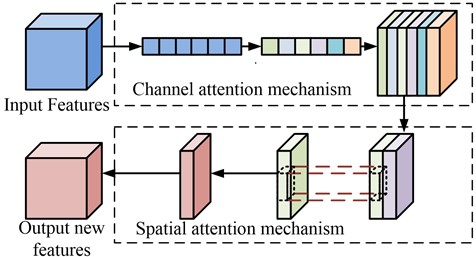
Fig. 1 shows the mixed AM. The operation object of the AM is the local information of the feature, which will maximize the search for complete local feature information during the operation. From Fig. 1, the mixed AM is composed of channel AM and spatial AM. Channel AM is often used for two-dimensional image processing. By establishing image channels, the dimensions of different feature information are compressed, and then the compressed features are compared with the original features to obtain the differences in features and differentiate them accordingly [14]. The spatial AM extends the computational level of the channel AM. After the channel AM completes feature classification based on differences, the spatial AM will confirm the spatial position of the feature and find the area containing the most feature information.

The AM used in this study is the mixed AM. The mixed AM can not only classify high and low-level fault features based on feature differences, but also determine the location of low-level features and extract them to complete the collection of low-level feature information [15]. Firstly, it is necessary to construct a basic feature extraction model based on the existing source domain fault features, and then input the feature information of the target domain to the model. To effectively distinguish between high and low-level features inputted into the target domain, it is necessary to establish a feature classification module using AM in the basic model. The first step in establishing this module is to construct a channel sub-module based on the channel AM. This sub-module is divided into a source domain containing existing feature data and a target domain containing the data to be tested. Assuming that the feature data in the source domain is $y_{t}$ , all feature sets in the source domain are $y_{s}$ , and $Y_{i}$ denotes the tensor of the $i$ th feature in the source domain. The feature data of the target domain is $m_{t}$ ; $M_{i}$ is the tensor of the $i$ th feature in the target domain. The expression for the feature sets of the source and target domains is Eq. (1):

1

\{\begin{array}{l} y_{s} = [y_{1}, y_{2}, . . . y_{t}], \\ m_{s} = [m_{1}, m_{2}, . . . m_{t}] . \end{array}

Fig. 2Channel module schematic

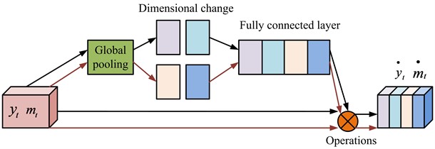
Fig. 2 is a schematic diagram of the channel module, from which the number of channels in this module is 2. The calculation is to first input the feature information of the source and target domains into the global pool, extract the features, then average the dimensions of the information, and then input the processed features with the same dimensions into the fully connected layer. After weight calculation and mapping function operation, the final feature data ${\dot{y}}_{t}$ and ${\dot{m}}_{t}$ are obtained. The expression for calculating the weight ratio of the source and the target domains is shown in Eq. (2):

2

\{\begin{array}{l} W_{y} = α (k (R e L U (Y_{i}))), \\ W_{m} = α (k (R e L U (M_{i}))) . \end{array}

In Eq. (2), $W_{y}$ and $W_{m}$ are the weight ratios of input feature channels in the source and target domains, respectively. $α$ means the sigmoid function. $k$ denotes the dimension. $R e L U$ is the activation function. After obtaining the weight ratio in the two domains, mapping operations can be performed based on the weight ratio and the original feature tensor to obtain the final input channel feature data. The mapping expression is shown in Eq. (3):

3

\{\begin{array}{l} {\dot{y}}_{t} = W_{y} \times Y_{t}, \\ {\dot{m}}_{t} = W_{m} \times M_{t} . \end{array}

After completing the classification of different domain features through the channel module, the spatial module can be established. The spatial module is operated on the theoretical basis of spatial AM, and compared to the channel module, the spatial module focuses more on the spatial dimension importance of features.

Fig. 3 shows the spatial module operation. From the figure, this operation first performs maximum and average pooling operations on the results obtained by the channel module, and then performs spatial weight ratio calculation and mapping operations again to obtain the final spatial feature output values ${\overset{*}{y}}_{t}$ and ${\overset{*}{m}}_{t}$ . The calculation of spatial weight ratio is shown in Eq. (4):

4

\{\begin{array}{l} {\overset{*}{W}}_{y} = α (f (M a x p o o l ({\dot{y}}_{t}); A v g p o o l ({\dot{y}}_{t}))) \\ {\overset{*}{W}}_{m} = α (f (M a x p o o l ({\dot{m}}_{t}); A v g p o o l ({\dot{m}}_{t}))) \end{array}

In Eq. (4), ${\overset{*}{W}}_{y}$ and ${\overset{*}{W}}_{m}$ are divided into spatial weight ratios of source and target domain features. $f$ is a convolutional function. By mapping the obtained feature space weight ratio with the input channel feature vector can obtain the final spatial feature tensor. The expression is shown in Eq. (5):

5

\{\begin{array}{l} {\overset{*}{y}}_{t} = {\overset{*}{W}}_{y} \times {\dot{y}}_{t}, \\ {\overset{*}{m}}_{t} = {\overset{*}{W}}_{m} \times {\dot{m}}_{t} . \end{array}

The channel and spatial modules constructed through AM can not only extract high-level features of bearing faults, but also recognize and classify low-level features. And the combination of the two modules can also reduce the differences between different levels of fault features.

Fig. 3Space module operation flow

3.2. CDFD model based on MLP-mixer

In the CDFD of bearings, due to the diverse reasons for mechanical equipment failures, the situations that require classification processing in diagnosis are also more complex. The AM model constructed in the study can effectively reduce the feature differences between different domains for feature classification and extraction. However, no clear solution has been provided for the transferability of features. To efficiently solve the feature transferability in CDFD, this study adds two feature correction modules using MLP-Mixer on the basis of the AM model to improve the transferability of cross domain fault features [16].

Fig. 4MLP-Mixer computing flow chart

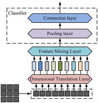
Fig. 4 shows the operational process of MLP-Mixer which is a technical framework that adopts multi-layer perception mechanism in computer vision technology, mainly including dimension conversion, feature mixing, pooling and connection layers. Among them, the pooling and connection layer functions together form a classifier for feature classification. The function of the dimension conversion layer is to convert the dimensions of features for subsequent feature fusion. The function of the feature mixing layer is to locally fuse information from different spatial positions. The classifier composed of pooling and connection layers is used to classify the fused information features according to their differences [17].

Due to the strong discriminative ability of the MLP-Mixer to the information features, its application in bearing fault diagnosis is based on this method to construct a fault diagnosis model under feature correction. The module is mainly divided into three steps, namely image segmentation, processing, and correction. It assumes that the target domain features input by the feature correction module are $t_{p}$ and the corresponding feature set is $t_{s}$ . The expression of $t_{s}$ is shown in Eq. (6):

6

t_{s} = [t_{1}, t_{2}, . . . t_{p}] .

The input feature of the source domain is $l_{p}$ , and the corresponding feature set is $l_{s}$ . The expression of $l_{s}$ is shown in Eq. (7):

7

l_{s} = [l_{1}, l_{2}, . . . l_{p}] .

The number of channels for feature transfer in this module is 2, with $D$ and $M$ being the corresponding two channel dimensions.

Fig. 5Fault diagnosis model built by MLP-Mixer

Fig. 5 shows a CDFD model constructed using MLP-Mixer. This model first divides the fault image into $N$ image blocks according to different dimensions. Then, an image processing layer is used to process the information of the fault image, and the processed image is input into the MLP-Mixer layer to obtain more complete image information. To improve the transferability of image features in the target domain, two feature correction modules are set up before feature output. By distinguishing between the corrected target source image and the processed source domain image based on the difference in image information, the vector matrix expression of the target source image information can be obtained as Eq. (8):

8

t_{s} = [\begin{array}{l} \begin{array}{l} {\dot{t}}_{1} & . . . & {\dot{t}}_{p}^{D} \end{array} \\ \begin{array}{l} . . . & \begin{array}{l}  \end{array} & . . . \end{array} \\ \begin{array}{l} {\dot{t}}_{s N}^{} & . . . & {\dot{t}}_{s N}^{D} \end{array} \end{array}] .

In Eq. (8), ${\dot{t}}_{1}$ is the first of the segmented $D$ dimension image matrix vector, and ${\dot{t}}_{p}^{D}$ is the last of the first row vector of the $D$ dimension image matrix. ${\dot{t}}_{s N}^{}$ means the last column vector in the first column, and ${\dot{t}}_{s N}^{D}$ denotes the last vector of the matrix. Among them, each image block represents different feature information.

Fig. 6Information fusion method

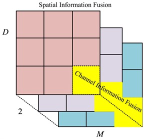
Fig. 6 shows the interaction method of image information. The information exchange method of different channels in the same space is called channel information exchange. The information exchange method in the same channel and different spaces is spatial information exchange. In the image information vector matrix containing the target domain, row vector can conduct channel information interaction, and column vector can conduct spatial information interaction. The information exchange is the image processing. After completing the image processing of the target domain, the processed feature data can be input into the feature correction module. The feature correction module is mainly composed of a fully connected layer and ReLU function, which can correct the feature differences between the target domain and the source domain to solve the reduced feature transferability. It assumes that the target and source domain feature values of the first feature correction module are $H (t_{p})$ and $H (l_{p})$ , respectively. The difference between the two features is $Δ H^{1} (p)$ . The expression for outputting the target source feature correction value is shown in Eq. (9):

9

{\bar{H}}^{1} (t_{p}) = Δ H^{1} (p) + H (t_{p}) .

In Eq. (9), ${\bar{H}}^{1} (t_{p})$ is the output target source feature correction value of the first correction module. This value is used as the input value for the second feature correction module, which corrects the target domain feature values $H (l_{p})$ and ${\bar{H}}^{1} (t_{p})$ with a difference value of $Δ H^{2} (p)$ . The expression for the final cross domain difference correction value obtained is shown in Eq. (10):

10

{\bar{H}}^{2} (t_{p}) = Δ H^{2} (p) + {\bar{H}}^{1} (t_{p}) .

In Eq. (10), ${\bar{H}}^{2} (t_{p})$ is the final feature difference correction result between the target domain and the source domain. In summary, the fault diagnosis model constructed through MLP-Mixer can achieve cross domain feature differentiation balance by extracting and correcting spatial and channel information of features. When the differences in features between different domains are balanced, the error caused by cross domain transfer will be reduced and the transferability of features will be improved during CDFD.

4. Analysis of CDFD model based on AM and MLP-Mixer

This study used a mixed AM and the MLP-Mixer algorithm to construct two models. One was a multi-domain feature classification model constructed through the mixed AM. This model completed the search for high and low-level features of faults by classifying the differences in local feature information. Therefore, this type of model needed to conduct performance analysis by judging its accuracy and the fault feature signals it searched for. The other was a feature correction fault diagnosis model constructed using the MLP-Mixer algorithm. This model improved the transferability of features by performing differential classification and balancing on cross domain fault features. Therefore, the performance of such models needed to be analyzed based on the accuracy, iteration times, and loss rate of fault diagnosis.

4.1. Design of experimental platform for bearing failure

In order to determine the performance of the bearing fault diagnosis model proposed in the study, a simulation experimental bench was designed and constructed. The test bench consists of an electric motor, a rack and pinion, a rotating shaft, a bearing steering and a load-bearing block. The coordinated operation between the rack and pinion and the rotating shaft is utilized to realize the operation of the experimental bench under the power provided by the electric motor. At the same time, the load-bearing block can simulate the actual shaft bearing force.

4.2. Rolling bearing fault signal vibration acquisition and measurement system design

The experiment uses the uT2502 wireless environmental excitation experimental modal test system for the vibration system, which is mainly composed of SR150M model sensors, signal receivers and computer systems containing analysis software. uT2502 vibration system has a built-in sensor signal acquisition range of 0-500 Hz, and an external sensor measurement frequency range of 0.1-10000 Hz. embedded hardware Integration circuit, can be directly realized multi-grade data measurement. Therefore, the sensor can meet the rolling bearing vibration signal acquisition. The signal receiver is uT3704FRS-ICP, with a sampling frequency of 51.2 kHz. The signal receiver is connected to the sensor, and after receiving the signals from the sensor, it will pass them to the computer system, which can analyze the data through the analysis software. The analysis software is added to the research to propose the corresponding detection algorithm module.

5. Experimental program design

The aim of this study is to evaluate the feature extraction models constructed using AMs. The performance evaluation was done using Convolutional Neural Network (CNN), Deep Domain Confusion (DDC) and Improved Convolutional Neural Network (TLCNN) algorithms for comparison where CNN has excellent feature recognition, DDC has domain feature search, and TLCNN has signal recognition capability. Four algorithmic modules are added to the uT2502 vibration system for detection of each. The SKF bearing dataset from Case Western Reserve University was chosen for this experiment, which is favorable for fault feature extraction because it has a high signal-to-noise ratio. The dataset contains four types of bearing data: internal structure failure, external structure failure, rolling ball failure and normal bearing. The specific types of fault features are shown in Table 1.

Table 1Bearing failure classification

Bearing failure type	Fault content	Fault number
Rolling ball failure	Ball breakage	F1
Internal structural failure	Cracks in the internal structure	F2
External structural failure	Cracks in the external structure	F3
Normal bearing	Difficult to run bearings	F4

Table 1 shows the classification of bearing faults for this experimental study. Where, different fault types were labeled for subsequent ease of analysis, and the four algorithmic models described above were used to determine bearing faults.

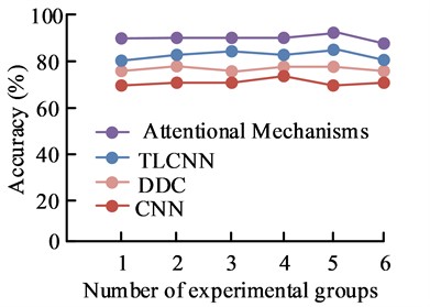
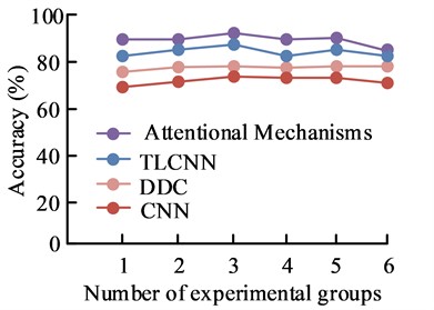
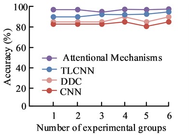
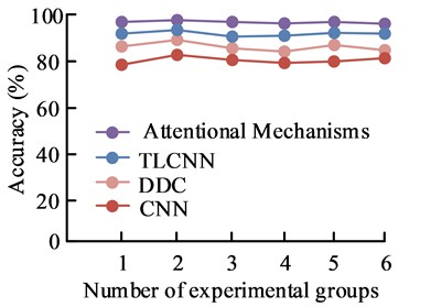
Fig. 7Recognition accuracy of four algorithms under four fault types

a)

b)

c)

d)

Fig. 7 shows the comparison of recognition accuracy of four algorithms in four types of bearing faults. Among them, Figs. 7(a), (b), (c), and (d) respectively show the recognition accuracy of the four algorithms under four types of faults: F1, F2, F3, and F4. Under the four types of fault identification, the model constructed using AM algorithm had the highest recognition accuracy, while the CNN algorithm had the lowest recognition accuracy. The recognition accuracies of the AM algorithm were 92.6 %, 91.2 %, 96.8 % and 97.3 % for the four bearing fault types F1, F2, F3 and F4, respectively. This was because the fault feature recognition model constructed using AM could not only effectively recognize signals from high-level features, but also extracted signals from low-level features, reducing the error in bearing fault feature recognition. Therefore, the feature recognition model constructed using AM had good application performance.

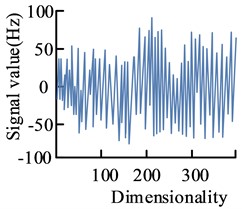
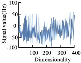
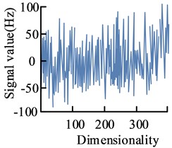
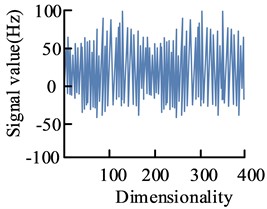
Fig. 8 shows the signal values of AM in fault diagnosis. Among them, Figs. 8(a), (b), (c) and (d) show the detected signal values of the bearings in states F1, F2, F3 and F4, respectively. It can be seen that the fluctuation range and trend of the detected signal values of the bearings in different states are different. The signal values of the bearings in the normal state are uniform, while the signal values corresponding to different faults have certain fluctuations. This was because the channel AM could distinguish the differences in feature information, and the spatial AM could determine the position of features. The combination of the two could obtain comprehensive feature information. This indicated that in actual bearing fault diagnosis, AM could effectively collect feature information and identify signal values of different faults. Therefore, AM had certain practical application value in bearing fault diagnosis.

Fig. 8Fault diagnosis signal values under the AM model

a)

b)

c)

d)

5.1. CDFD model based on MLP-Mixer

To verify the performance of the fault diagnosis model constructed using MLP-Mixer, this study used envelope frequency transfer component analysis (ET-TCA), with DDC and CNN as comparative algorithms. Among them, ET-TCA had the function of aligning source and target domain features. The domain feature search function of DDC could search for cross domain features with high similarity. CNN could identify the differences in features and predict fault types. This experiment used the above four algorithms to diagnose and analyze the four types of faulty bearings in Table 1. And it compared performance based on the accuracy, iteration times, and loss rate of fault diagnosis.

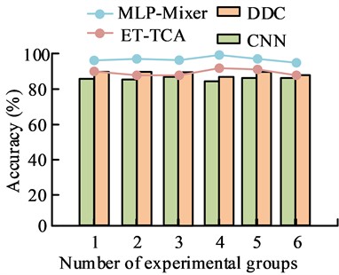
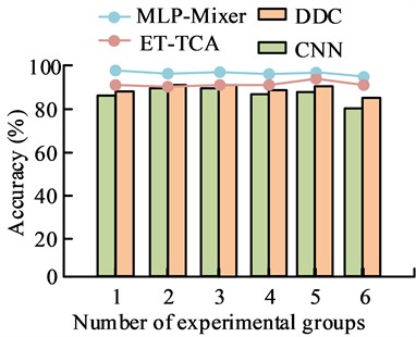
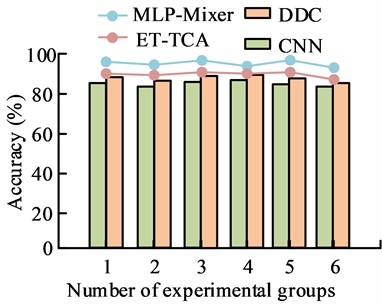
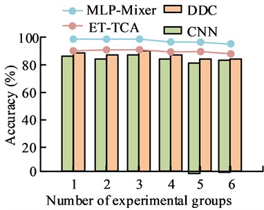
Fig. 9 shows the accuracy of the bearing condition diagnostic model with the four detection models. Among them, Figs. 9(a), (b), (c) and (d) show the diagnostic accuracies of the four modified algorithms for the four fault types F1, F2, F3 and F4, respectively. The MLP-Mixer algorithm has the highest accuracy in recognizing the four fault types, while the CNN algorithm has the lowest accuracy. The MLP-Mixer has the highest accuracy for the four bearing types and can achieve 98.8 %, 97.9 %, 98.9 %, and 99.5 % for the F1, F2, F3, and F4 states, respectively. This was because the MLP-Mixer fault diagnosis model had two correction modules, which could reduce the feature differences between different domains, make the expression of information content more specific, and improve the transferability of cross domain features. Therefore, the MLP-Mixer model had effective feature correction ability and had certain application value in fault diagnosis.

Fig. 10 shows the iteration times of four correction algorithms. From Fig. 10, all four algorithms could reach a stable state after varying degrees of convergence speed. Among them, MLP-Mixer algorithm had the fastest convergence speed. When it iterated to the 26th generation, it converged to a stable state. At this time, the algorithm had the ability of stable optimization, and the stable fitness value was 0.27. The CNN algorithm had the slowest convergence speed. It started to converge to a stable state when it iterated to the 32nd generation. At this time, the stable fitness value was 0.35. Therefore, the MLP-Mixer algorithm had a certain ability to search for optimal values, which could effectively search for characteristic values with differences to achieve the effect of balancing the differences in cross domain features. Therefore, the MLP-Mixer algorithm had good feature correction ability.

Fig. 9Accuracy of bearing condition diagnostic model with four detection models

a)

b)

c)

d)

Fig. 10Number of iterations of the four calibration algorithms

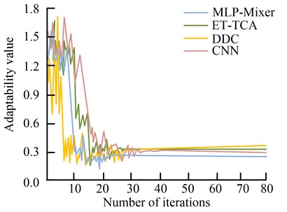
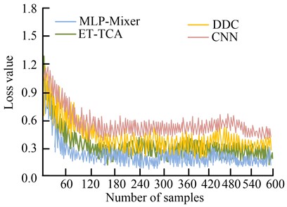
Fig. 11 shows the loss curves of four correction algorithms. From the graph, the loss values of the four correction algorithms first decreased and then gradually stabilized as the number of samples increased. Among them, the MLP-Mixer algorithm had the fastest loss curve to reach a stable state, the smallest loss value at stability, and a stable loss value of 0.28. Next was ET-TCA, with a stability loss value of 0.30, followed by DDC, with a stability loss value of 0.41. The CNN algorithm had the highest stability loss value, which could reach 0.58. In summary, the MLP-Mixer algorithm had a higher degree of loss in the computation than the other three algorithms.

Fig. 11Loss curves for the four correction algorithms

6. Conclusions

The structural composition of modern mechanical equipment is relatively complex, and the operation are closely connected. As the core component for safe operation of equipment, the safety performance of rolling bearings is of certain importance. Although traditional bearing CDFD methods can perform fast operations, their recognition accuracy is relatively low. To address the above issues, this study first adopted a mixed AM to construct a cross domain feature extraction model. Through this model, different layers of features were recognized, classified, and extracted to improve the comprehensiveness of feature extraction. Then, a CDFD model was constructed based on the MLP-Mixer algorithm, with the extracted feature signal values as input and two feature correction modules added to balance the differences between different domains. The experimental results showed that the highest recognition accuracy of the AM model for different fault types was 92.6 %, 91.2 %, 96.8 % and 97.3 %, respectively, which was higher than the other three comparative algorithms. Moreover, the model could successfully extract the corresponding global signal values. This indicated that compared to other algorithms, the model had excellent feature recognition and extraction capabilities. The highest recognition accuracy of the MLP-Mixer model for four types of faults was 98.8 %, 97.9 %, 98.9 % and 99.5 %, respectively, which was superior to the other three correction algorithms. And the model could converge to a stable state when it iterated to the 26th generation. The stability fitness value was 0.27, and the stability loss value was 0.28, which showed that the model had good feature optimization ability. Liu et al. used a combination of generative adversarial nets and feature matching for fault detection of rotary bearings. The average detection accuracy of this method could reach 98.36 %, and the study proposed that the accuracy of the approach was slightly better than the generative adversarial nets method [18]. Therefore, the two models proposed in the article have good application value in rolling bearing fault diagnosis, and the performance of this model can be verified by increasing the number of domains in the future.

References

K. I.-K. Wang, X. Zhou, W. Liang, Z. Yan, and J. She, “Federated transfer learning based cross-domain prediction for smart manufacturing,” IEEE Transactions on Industrial Informatics, Vol. 18, No. 6, pp. 4088–4096, Jun. 2022, https://doi.org/10.1109/tii.2021.3088057

Publisher
S. Han, S. Oh, and J. Jeong, “Bearing fault diagnosis based on multiscale convolutional neural network using data augmentation,” Journal of Sensors, Vol. 2021, pp. 1–14, Feb. 2021, https://doi.org/10.1155/2021/6699637

Publisher
Z. Chai, C. Zhao, and B. Huang, “Multisource-refined transfer network for industrial fault diagnosis under domain and category inconsistencies,” IEEE Transactions on Cybernetics, Vol. 52, No. 9, pp. 9784–9796, Sep. 2022, https://doi.org/10.1109/tcyb.2021.3067786

Publisher
Z. Huang et al., “A multisource dense adaptation adversarial network for fault diagnosis of machinery,” IEEE Transactions on Industrial Electronics, Vol. 69, No. 6, pp. 6298–6307, Jun. 2022, https://doi.org/10.1109/tie.2021.3086707

Publisher
Q. Liu, H. Sun, Y. Chai, J. Zhu, T. Wang, and X. Qing, “On-site monitoring of bearing failure in composite bolted joints using built-in eddy current sensing film,” Journal of Composite Materials, Vol. 55, No. 14, pp. 1893–1905, Jun. 2021, https://doi.org/10.1177/0021998320979737

Publisher
H. Tang, H.-L. Dai, and Y. Du, “Bearing fault detection for doubly fed induction generator based on stator current,” IEEE Transactions on Industrial Electronics, Vol. 69, No. 5, pp. 5267–5276, May 2022, https://doi.org/10.1109/tie.2021.3080216

Publisher
P. Wang, D. Li, and N. Zhang, “Research on early warning of rolling bearing wear failure based on empirical mode decomposition,” International Journal of Materials and Product Technology, Vol. 63, No. 1/2, p. 72, 2021, https://doi.org/10.1504/ijmpt.2021.117036

Publisher
F. Yin, W. Lu, S. Nie, F. Lou, H. Ji, and Z. Ma, “Failure analysis and improvement of the tribological performance of sliding bearing tribopair in integrated energy recovery-pressure boost device,” Ceramics International, Vol. 47, No. 21, pp. 30367–30380, Nov. 2021, https://doi.org/10.1016/j.ceramint.2021.07.217

Publisher
B. Cui, Y. Weng, and N. Zhang, “A feature extraction and machine learning framework for bearing fault diagnosis,” Renewable Energy, Vol. 191, pp. 987–997, May 2022, https://doi.org/10.1016/j.renene.2022.04.061

Publisher
W. Zhang, X. Li, H. Ma, Z. Luo, and X. Li, “Open-set domain adaptation in machinery fault diagnostics using instance-level weighted adversarial learning,” IEEE Transactions on Industrial Informatics, Vol. 17, No. 11, pp. 7445–7455, Nov. 2021, https://doi.org/10.1109/tii.2021.3054651

Publisher
L. Chen, Q. Li, C. Shen, J. Zhu, D. Wang, and M. Xia, “Adversarial domain-invariant generalization: A generic domain-regressive framework for bearing fault diagnosis under unseen conditions,” IEEE Transactions on Industrial Informatics, Vol. 18, No. 3, pp. 1790–1800, Mar. 2022, https://doi.org/10.1109/tii.2021.3078712

Publisher
Z. Wang, X. He, B. Yang, and N. Li, “Subdomain adaptation transfer learning network for fault diagnosis of roller bearings,” IEEE Transactions on Industrial Electronics, Vol. 69, No. 8, pp. 8430–8439, Aug. 2022, https://doi.org/10.1109/tie.2021.3108726

Publisher
Y. Yao, B. Gu, M. Alazab, N. Kumar, and Y. Han, “Integrating multihub driven attention mechanism and big data analytics for virtual representation of visual scenes,” IEEE Transactions on Industrial Informatics, Vol. 18, No. 2, pp. 1435–1444, Feb. 2022, https://doi.org/10.1109/tii.2021.3089689

Publisher
X. Zhao, M. Qi, Z. Liu, S. Fan, C. Li, and M. Dong, “End‐to‐end autonomous driving decision model joined by attention mechanism and spatiotemporal features,” IET Intelligent Transport Systems, Vol. 15, No. 9, pp. 1119–1130, Sep. 2021, https://doi.org/10.1049/itr2.12086

Publisher
Y. Guo, Z. Mustafaoglu, and D. Koundal, “Spam detection using bidirectional transformers and machine learning classifier algorithms,” Journal of Computational and Cognitive Engineering, Vol. 2, No. 1, pp. 5–9, Apr. 2022, https://doi.org/10.47852/bonviewjcce2202192

Publisher
M. H. Farrell, T. Liang, and S. Misra, “Deep neural networks for estimation and inference,” Econometrica, Vol. 89, No. 1, pp. 181–213, 2021, https://doi.org/10.3982/ecta16901

Publisher
F. Amato, L. Coppolino, F. Mercaldo, F. Moscato, R. Nardone, and A. Santone, “CAN-bus attack detection with deep learning,” IEEE Transactions on Intelligent Transportation Systems, Vol. 22, No. 8, pp. 5081–5090, Aug. 2021, https://doi.org/10.1109/tits.2020.3046974

Publisher
S. Liu, J. Chen, S. He, E. Xu, H. Lv, and Z. Zhou, “Intelligent fault diagnosis under small sample size conditions via Bidirectional InfoMax GAN with unsupervised representation learning,” Knowledge-Based Systems, Vol. 232, p. 107488, Nov. 2021, https://doi.org/10.1016/j.knosys.2021.107488

Publisher

About this article

Received

19 June 2023

Accepted

26 September 2023

Published

30 October 2023

DOI

https://doi.org/10.21595/jme.2023.23460

Keywords

MLP-Mixer

attention mechanism

rolling bearing

fault diagnosis

cross domain

Acknowledgements

The research was supported by: Research and Practice Project of Higher Education Teaching Reform in Henan Province and Research and Practice of Smart Classroom Teaching Effect Evaluation Based on Teaching Diagnosis Reform (No. 2019SJGLX791).

Data Availability

The datasets generated during and/or analyzed during the current study are available from the corresponding author on reasonable request.

Conflict of interest

The authors declare that they have no conflict of interest.

This is an open access article distributed under the Creative Commons Attribution License, which permits unrestricted use, distribution, and reproduction in any medium, provided the original work is properly cited.

Previous article in issue Previous Next article in issue Next

Research article

2023 08 18

Fault diagnosis of rolling bearing based on cross-domain divergence alignment and intra-domain distribution alienation

Shubiao Zhao, Guangbin Wang, Xuejun Li, Jinhua Chen, Lingli Jiang

Research article

2023 08 01

A fault diagnosis method based on dilated convolution and attention for rolling bearing under multiple working conditions and noisy environments

Hui Zhang, Shengdong Liu, Ziwei Lv, Zhenlong Sang, Fangning Li

Review article

2021 11 26

Fault diagnosis and health management of bearings in rotating equipment based on vibration analysis – a review

Adnan Althubaiti, Faris Elasha, Joao Amaral Teixeira

Research article

2021 02 04

Research on fault diagnosis of rolling bearings based on conditional variance statistic and cross-correlation spectrum

Baoyu Huang, Yongxiang Zhang, Danchen Zhu

X. Mao, “Cross domain fault diagnosis method based on MLP-mixer network,” Journal of Measurements in Engineering, Vol. 11, No. 4, pp. 453–466, Oct. 2023, https://doi.org/10.21595/jme.2023.23460

Copy Extrica

Copied to clipboard!

TY  - JOUR
DO  - 10.21595/jme.2023.23460
UR  - https://doi.org/10.21595/jme.2023.23460
TI  - Cross domain fault diagnosis method based on MLP-mixer network
T2  - Journal of Measurements in Engineering
AU  - Mao, Xiaodong
PY  - 2023
DA  - 2023/10/30
PB  - JVE International Ltd.
SP  - 453-466
VL  - 11
IS  - 4
SN  - 2335-2124
SN  - 2424-4635
ER  - 

Copy Ris

Copied to clipboard!

 @article{Mao_2023, title={Cross domain fault diagnosis method based on MLP-mixer network}, volume={11}, ISSN={2424-4635}, url={https://doi.org/10.21595/jme.2023.23460}, DOI={10.21595/jme.2023.23460}, number={4}, journal={Journal of Measurements in Engineering}, publisher={JVE International Ltd.}, author={Mao, Xiaodong}, year={2023}, month=oct, pages={453–466} }

Copy Bibtex

Copied to clipboard!

[1]X. Mao, “Cross domain fault diagnosis method based on MLP-mixer network,” Journal of Measurements in Engineering, vol. 11, no. 4, pp. 453–466, Oct. 2023, doi: 10.21595/jme.2023.23460.

Copy IEEE

Copied to clipboard!

Mao, Xiaodong. “Cross Domain Fault Diagnosis Method Based on MLP-Mixer Network.” Journal of Measurements in Engineering 11, no. 4 (October 30, 2023): 453–66. https://doi.org/10.21595/jme.2023.23460.

Copy Chicago

Copied to clipboard!

Cross domain fault diagnosis method based on MLP-mixer network

Abstract

1. Introduction

2. Related works

3. CDFD of bearings based on AM and MLP-Mixer

3.1. Constructing a multi-domain fault feature extraction model based on AM

3.2. CDFD model based on MLP-mixer

4. Analysis of CDFD model based on AM and MLP-Mixer

4.1. Design of experimental platform for bearing failure

4.2. Rolling bearing fault signal vibration acquisition and measurement system design

5. Experimental program design

5.1. CDFD model based on MLP-Mixer

6. Conclusions

References

About this article

Related Articles