Active suspension LQR control based on modified differential evolutionary algorithm optimization

Zou, Junyi; Zuo, Xinkai

doi:10.21595/jve.2024.23953

Journal of Vibroengineering

Browse Journal

Submit article

Published: 27 May 2024

Check for updates

Active suspension LQR control based on modified differential evolutionary algorithm optimization

Junyi Zou¹

Xinkai Zuo²

^{1, 2}Wuhan University of Science and Technology, Wuhan, Hubei, China

Corresponding Author:

Junyi Zou

Cite the article Download PDF

Article in Press

Downloads 40

Abstract

The selection of weight matrices Q and R in the LQR control strategy for active suspension is susceptible to subjective interference. To address this issue, a modified differential evolutionary algorithm is proposed to optimize the active suspension LQR controller, ensuring that the weighting coefficients are set to their optimal values. The differential evolutionary algorithm exhibits drawbacks in terms of its slow convergence rate and the significant impact of algorithm parameter settings on the obtained results. An modified differential evolutionary algorithm that is adaptive to the two candidate mutation strategies and adaptively adjusts the scaling factor and crossover rate is proposed so as to better improve the ability of jumping out of the local optimum and global search. The algorithm's functionality is verified by constructing a 1/4 suspension model in the Simulink software platform and implementing a modified differential evolution algorithm program written in C++ language using MATLAB. The program iterates through Simulink inputs to obtain the optimal fitness value for three suspension comfort indices. By comparing the results with those obtained from passive suspension and traditional LQR control of active suspension, optimizing the LQR control of active suspension based on the modified differential evolution algorithm can effectively reduce vehicle vibration amplitude while considering overall suspension performance enhancement, thereby significantly improving ride comfort and handling stability.

Active suspension LQR control based on modified differential evolutionary algorithm optimization

Highlights

An active suspension LQR control based on an improved differential evolutionary algorithm is presented.
The improved differential evolutionary algorithm implements mutation strategy adaptive, scaling factor and crossover rate adaptive adjustment.
After optimizing the LQR using the algorithm, the body sag acceleration, suspension dynamic travel and tire dynamic displacement were optimized by 1.6%, 27.1% and 6.6%, respectively.
A more optimal trade-off between the weighting matrices Q and R is realized, which improves the ride comfort and handling stability of the vehicle.

1. Introduction

Automobile is one of the most important means of transportation in modern society, and the driving and riding experience of automobile has received more and more attention. The main components of the automobile suspension system are springs, shock absorbers and guiding mechanisms, which connect the body and wheels and attenuate the body vibration caused by the road excitation. Excessive vibration intensity may damage the system structure to a certain extent [1, 2]. Suspension system of vehicle ride comfort and security has an important influence, and is one of the key systems that determine vehicle dynamic performance [3]. Lately, with the development of automotive electronic technology and automotive intelligence, the application of MCU in vehicles has become increasingly common, coupled with the maturity and wide range of components technology such as adjustable shock absorber, air spring and vehicle sensor, advanced suspension system has received extensive attention and research. The controllable suspension, also referred to as "intelligent suspension" by certain automobile manufacturers, is capable of dynamically adjusting the damping or stiffness of the suspension based on the current driving conditions. This feature enhances the performance of the suspension system to a certain extent and mitigates the inherent trade-off between comfort and safety [4].

The quality of suspension system will directly affect the driving experience and the occupant's subjective comfort feeling. There are three kinds of automobile suspension systems: passive suspension, semi-active suspension and active suspension [5]. The component parameters and performance of traditional passive suspension are fixed, lacking the ability to adjust for different driving conditions, thereby compromising comfort and handling stability under varying circumstances. To enhance automobile suspension performance, active suspension systems were introduced as a solution. By utilizing hydraulic actuators, linear motors, and other technologies, active suspension replaces or works in parallel with the springs and shock absorbers of passive suspension systems to generate corresponding forces based on control signals [6]. The active suspension system surpasses the limitations imposed by passive systems and provides a broad range of adjustable output. The use of appropriate control methods in the suspension system to reduce the vibration amplitude of the vehicle and improve the ride experience for passengers is the current research hotspot in the field of automobile suspension.

In terms of suspension system design, ever since the initial proposal by American professor Labrosse regarding the concept of suspension performance control, a series of active suspension prototypes have emerged successively, leading to the commercialization of numerous research findings that exhibit excellent control effects. The research on diverse fundamental control algorithms and their integrated control algorithms is currently thriving in the field of suspension control strategy. Scholars all over the world have introduced a variety of mature control technologies into the active suspension system of automobiles, such as PID control, LQG control [7]. Optimal control is a control method that selects one of several control methods to achieve the optimal objective function. It is widely used in the field of vehicle dynamics because of its high robustness, fast calculation speed and clear purpose in solving multi-variable and nonlinear problems. Linear quadratic regulator (LQR) control is a kind of relatively mature, relatively complete theory of optimal control method, which is widely used [8]. However, the control effect of this method depends largely on the weight coefficients of its performance indicators, and previous researchers have continuously adjusted the weights through human experience. In recent years, with the continuous development of intelligent algorithms, many researchers have begun to introduce intelligent algorithms in active suspension control. He et al. used genetic algorithm to improve the LQR controller and Kalman filter in the vehicle combination system to improve the overall performance of the vehicle system; Jiao Rui et al. introduced adaptive differential evolutionary algorithm to optimize the single-neuron PID control and to improve the vehicle suspension’s vertical acceleration of the vehicle body performance index to improve ride comfort. Oral Ö, Çetin L and Uyar E proposed a method to solve the optimal control problem, in which the $Q$ and $R$ matrices are derived by time-domain computation, but the weighting parameters need to be adjusted. Chen Xiaobing et al. introduced a differential evolutionary algorithm to optimize the LQR controller of the active suspension to optimize the comfort of the ride, the stability of the driving and the safety, but the algorithm optimization process was slow, and the system convergence was not satisfactory.

The differential evolutionary algorithm, being one of the classical intelligent algorithms, possesses the advantages of a limited number of control parameters, excellent convergence properties, and robust optimization capabilities [9]. Therefore, when dealing with optimization problems with constraints, many researchers have combined the Differential Evolution algorithm with the constraint process, and this algorithm has a stronger optimization ability than the genetic algorithm and greatly reduces the time complexity. However, the differential evolutionary algorithm also has problems such as slow convergence and large influence of algorithm parameters on the results [10].

Taking active suspension as the research object, this paper first built a two-degree-of-freedom suspension model in Matlab software, and then designed an LQR optimal control controller based on two-degree-of-freedom suspension. Due to the shortcomings of existing algorithms, a differential evolution algorithm based on adaptive scaling factor and adaptive cross probability was designed, and the excellence of the algorithm was verified by test functions. The optimization scheme is designed according to the fitness function, and the penalty function is added to quickly optimize the coefficients in the LQR matrix. Finally, the simulation results of passive suspension and traditional LQR suspension are compared, and the good effect of the proposed algorithm on LQR control optimization is proved.

2. Modeling of vehicle control system

2.1. Pavement modeling

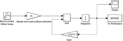
The first-order filtered band-limited white noise method is used to model the stochastic pavement excitation as shown in Eq. (1):

1

{\dot{x}}_{g} (t) = - 2 π f_{0} x_{g} (t) + 2 π \sqrt{G （n_{0}） ν} ω (t) .

The lower cut-off frequency is $f_{0}$ ; $x_{g} (t)$ is the pavement vertical displacement; $G (n_{0})$ is the pavement unevenness coefficient; $ν$ is for speed; The Gaussian white noise with zero expectation is $ω (t)$ .

Fig. 1Pavement excitation model

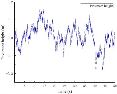
Take $f_{0}$ as 0.1, the speed is set to 20 m/s. The road unevenness coefficient $G (n_{0})$ is 5×10^-6. A 50 s section of simulated road condition is generated in MATLAB as shown in Fig. 2. The same section of road surface is input into the system during subsequent simulation.

Fig. 2Simulated road conditions

2.2. Active suspension modeling

To mitigate the influence of extraneous factors, simplify the suspension system for streamlined analysis, and effectively evaluate the true impact of the enhanced differential evolutionary algorithm on optimizing LQR control in active suspension systems, this study employs said algorithm to a 1/4 automobile active suspension model using MATLAB simulation platform.

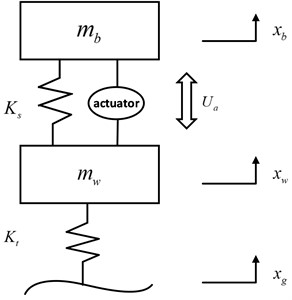
The mathematical model of active suspension is established to establish the theoretical basis for the analysis of vibration characteristics and control performance. The active suspension model is constructed as shown in Fig. 3. In Fig. 3, the spring loaded mass is $m_{b}$ ; The unsprung mass is $m_{w}$ ; The suspension stiffness is $K_{s}$ ; $K_{t}$ is the tire stiffness; The vertical displacement of the body is $x_{b}$ ; $x_{w}$ is the vertical displacement of the wheels; The vertical displacement of the road surface is $x_{g}$ and $U_{a}$ is the control force of the actuator [11].

Fig. 3Model diagram of active suspension

Differential equations are developed to describe the suspension model based on automotive vibration theory as well as Newton’s second law:

2

\{\begin{array}{l} m_{b} {\ddot{x}}_{b} = U_{a} - K_{s} (x_{b} - x_{w}), \\ m_{w} {\ddot{x}}_{w} = - U_{a} + K_{s} (x_{b} - x_{w}) - K_{t} (x_{w} - x_{g}) . \end{array}

Thus, the state variables of the system can be determined as:

3

x = {[{\dot{x}}_{b}, {\dot{x}}_{w}, x_{b}, x_{w}, x_{g}]}^{T} .

The body vertical acceleration $\ddot{x_{b}}$ , the suspension dynamic travel $(x_{b} - x_{w})$ and the tire dynamic displacement $(x_{w} - x_{g})$ are used as system output variables, i.e:

4

y = [{\ddot{x}}_{b}, x_{b} - x_{w}, x_{w} - x_{g}] .

Thus, to get the system state space equation:

5

\{\begin{array}{l} \dot{x} = A x + B u + G ω, \\ y = C x + D u, \end{array}

where: $u$ is the input matrix, $u = [U_{a} (t)]$ ; $ω$ is the white noise matrix, $ω = ω (t)$ ; $A$ , $B$ , $G$ , $C$ , and $D$ are coefficient matrices as follows:

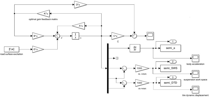
A = [\begin{array}{l} 0 & 0 & - \frac{K_{s}}{m_{b}} & \frac{K_{s}}{m_{b}} & 0 \\ 0 & 0 & \frac{K_{s}}{m_{w}} & - \frac{K_{t} + K_{s}}{m_{w}} & \frac{K_{t}}{m_{w}} \\ 1 & 0 & 0 & 0 & 0 \\ 0 & 1 & 0 & 0 & 0 \\ 0 & 0 & 0 & 0 & 2 π f_{0} \end{array}], B = [\begin{matrix} \frac{1}{m_{b}} \\ - \frac{1}{m_{w}} \\ 0 \\ 0 \\ 0 \end{matrix}], G = [\begin{matrix} 0 \\ 0 \\ 0 \\ 0 \\ 2 π \sqrt{G_{0} u} \end{matrix}],

C = [\begin{array}{l} 0 & 0 & \frac{K_{s}}{m_{b}} & \frac{K_{s}}{m_{b}} & 0 \\ 0 & 0 & 1 & - 1 & 0 \\ 0 & 0 & 0 & 1 & - 1 \end{array}], D = {[\begin{array}{l} \frac{1}{m_{b}} & 0 & 0 \end{array}]}^{T} .

The 1/4 active suspension system is modeled by deriving the equations mentioned above and specifying its inputs and outputs.

Fig. 4Active suspension model

3. LQR controller design

The automobile suspension LQR controller is designed to achieve effective suspension control with small inputs using the fitness function as an object. Three performance metrics for evaluating the suspension include body sag acceleration, tire dynamic displacement and suspension dynamic travel. In addition, it is also necessary to consider the control of energy consumption, so that the control energy consumption is small.

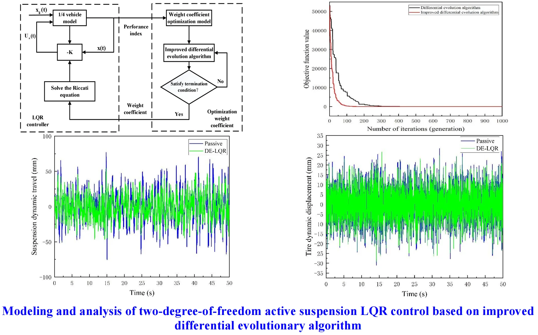
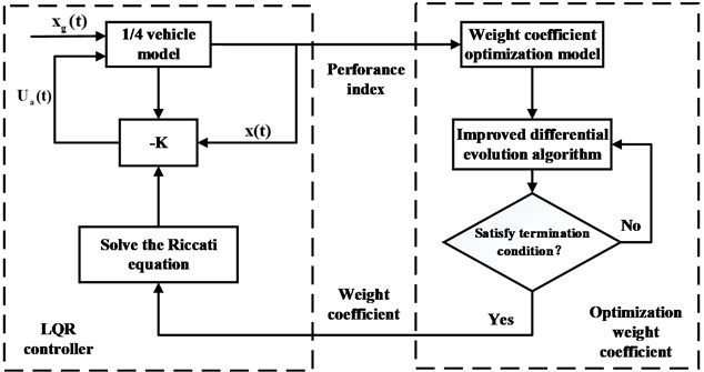
The principle of active suspension LQR control based on improved differential evolutionary algorithm is shown in Fig. 5.

Fig. 5Block diagram of LQR control of active suspension based on improved differential evolutionary algorithm

With the goal of improving the ride comfort of the car and at the same time ensuring the safe operation of the car, the optimization fitness function $J$ is determined as [12]:

6

J = \int_{0}^{\infty} [q_{1} (x_{w} - x_{g})^{2} + q_{2} (x_{b} - x_{w})^{2} + q_{3} {\ddot{x}}_{b}^{2}] d t .

Type: in $q_{1}$ and $q_{2}$ , $q_{3}$ respectively tire dynamic displacement body vertical acceleration, suspension dynamic schedule, weight coefficient.

Converting the above equation to matrix form, we have:

7

J = \int_{0}^{\infty} (x^{T} Q x + u^{T} R u + 2 x^{T} N u) d t,

where:

Q = [\begin{array}{l} 0 & 0 & 0 & 0 & 0 \\ 0 & 0 & 0 & 0 & 0 \\ 0 & 0 & q_{2} + \frac{q_{3} K_{s}^{2}}{m_{b}^{2}} & - q_{2} - \frac{q_{3} K_{s}^{2}}{m_{b}^{2}} & 0 \\ 0 & 0 & - q_{2} - \frac{q_{3} K_{s}^{2}}{m_{b}^{2}} & q_{1} + q_{2} + \frac{q_{3} K_{s}^{2}}{m_{b}^{2}} & - q_{1} \\ 0 & 0 & 0 & - q_{1} & q_{1} \end{array}], R = \frac{q_{3}}{m_{b}^{2}}, N = \frac{1}{m_{b}^{2}} [\begin{matrix} 0 \\ 0 \\ - q_{3} K_{s} \\ q_{3} K_{s} \\ 0 \end{matrix}] .

The optimal control force for LQR is:

8

U_{a} = - K x (t) .

Type: $x (t)$ for any time feedback state variables; $K$ for the optimal control feedback gain matrix.

According to Eq. (8), $K$ can be written:

9

K = - R^{- 1} B^{T} P x .

Type: $P$ for symmetric matrix.

Through Riccati differential equation, $P$ can be obtained as follows:

10

P A + A^{T} P - P B R^{- 1} B^{T} P + Q = 0 .

It can be seen that the effect of LQR control of active suspension completely depends on the weight matrix $Q$ and $R$ [13]. However, there is no specific method for determining these two matrices, and they usually rely on the experience of the designers to select them, which makes it difficult to ensure that the optimization parameters are in the optimal state, and it takes a long time. To address the aforementioned issues, this paper proposes utilizing a modified differential evolutionary algorithm to optimize the weight matrix parameters. This approach aims to mitigate the impact of subjective human factors on weight selection and further enhance its efficiency, resulting in a more rapid and effective process [14].

4. Modified differential evolution algorithm and design

4.1. Standard difference evolutionary algorithm

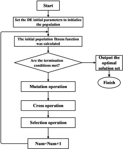
Differential evolution algorithm is a new optimization algorithm, which is developed on the basis of swarm intelligence theory [15]. It is a new type of intelligent optimization algorithm that uses the collaboration and competition between individuals in the swarm [16]. Differential evolutionary algorithm realizes the optimization search through two ways: one is based on the realization of mutation operation through difference, and the other is the crossover operation of the population through probabilistic random selection. Although the name of its operation is the same as that of the genetic algorithm, the realization method is fundamentally different. The basic principle is to randomly generate a population with a certain number of individuals, each individual is a vector representing a set of solutions to the optimization objective function, and then continuously update the individuals through mutation and crossover operations to increase the diversity of the population [17], and then through selection operations to eliminate the individuals with bad fitness values and retain the good ones, and then continuously approach the optimal solution through continuous iteration and computation, and find the optimal individual with the best fitness value can be found through continuous iteration and calculation [18].

The differential evolutionary algorithm process is specified as follows.

(1) Initialization of stocks. First starting from the NP random candidate solutions, usually a differential evolutionary population is formed by each individual for NP, remember to:

11

x_{_{i, G}} = (x_{1, G}, x_{2, G}, \dots, x_{D, G}), (i = 1,2, \dots, N P),

where is $N P$ population size, from the current group after generation of mutation and crossover and individual choice and the NP a test. This step consists of a cycle, until reach the end condition. Randomly generated initial population, as shown in Eq. (12):

12

x_{i, j} = x_{i, j}^{L} + r a n d (0,1) \times (x_{i, j}^{U} - x_{i, j}^{L}),

where, denotes the $j$ th component of the $i$ thindividual. $x_{i, j}^{L}$ , $x_{i, j}^{U}$ respectively the first $j$ a component of the lower bound and upper bound. $R a n d (0,1)$ said within the range of (0, 1) uniformly distributed random Numbers.

(2) Mutation operation. Differential strategies are the way in which differential evolutionary algorithms achieve individual variation, which is an important difference from genetic algorithms that exist. The difference between two random individuals and the scaling factor $F$ and the target vector generates a mutant individual. A mutant individual is generated from the difference of two random individuals with scaling factor F and target vector, and DE uses the difference strategy for individual mutation. Here are some common mutation strategies:

1) DE/rand/1:

13

v_{i, G} = x_{r 1, G} + F \times (x_{r 2, G} - x_{r 3, G}) .

2) DE/best/1:

14

v_{i, G} = x_{b e s t, G} + F \times (x_{r 1, G} - x_{r 2, G}) .

3) DE/current-to-best/1:

15

v_{i, G} = x_{i, G} + F \times (x_{b e s t, G} - x_{i, G}) + F \times (x_{r 1}, G - x_{r 2, G}) .

4) DE/current-to-rand/1:

16

v_{i, G} = x_{i, G} + r a n d \times (x_{r 1, G} - x_{i, G}) + F \times (x_{r 2, G} - x_{r 3, G}),

where $r_{1}$ , $r_{2}$ , and $r_{3}$ are index subscripts that represent three mutually unequal individuals randomly selected from the population. $F$ is the scaling factor that controls the strength of the difference [19]. $x_{b e s t}$ represents the one which has the best fitness value of individual.

(3) Cross-operation. To increase the diversity of the population, the variant vector and the parent vector are both combined to produce new candidate solutions and eventually a new test vector. The crossover operation between the $g$ th generation individuals of $x_{i, G}$ and the intermediate individuals of the variant $υ_{i, G}$ :

17

u_{i, j, G} = \{\begin{array}{l} ν_{i, j, G}, r a n d \leq C R o r j = j_{r a n d}, \\ x_{i, j, G}, o t h e r w i s e, \end{array}

where $C R$ is the crossover probability, which determines the proportion of heredity among different individuals. $j_{r a n d}$ is a random integer in $[1,2 \dots, D]$ .

(4) Selection of operations. The selection operation in the differential evolutionary algorithm employs a greedy approach to choose the individual with the optimal function value for inclusion in the next generation:

18

x_{i, G + 1} = \{\begin{array}{l} u_{i, G}, f (u_{i, G}) \leq f (x_{i, G}), \\ x_{i, G}, o t h e r w i s e . \end{array}

Differential evolutionary algorithm flow chart is as follows.

Fig. 6Differential evolution algorithm flow chart

4.2. Differential evolution algorithm optimization strategy

In standard differential evolution optimization algorithm, the scaling factor $F$ and crossover probability $C R$ take fixed values, however, it is more difficult to determine an appropriate parameter in the optimization process [20]. As the scaling factor $F$ increases, the degree of population differentiation decreases, and the phenomenon of local extremes in evolution occurs, causing the population to converge prematurely. When the scaling factor $F$ is larger, it is less likely to fall into local extremes, but its convergence speed will be slower. The crossover probability $C R$ can effectively control the participation of each dimensional parameter value in the crossover process, and at the same time take into account the global and local optimization ability. As the crossover probability $C R$ decreases, the diversity of the population decreases, which easily leads to premature convergence. As the value of $C R$ increases, the convergence of the algorithm increases. However, the crossover probability is too large so that its convergence slows down due to the size of the disturbance exceeding the degree of population differentiation.

Based on the above problems, the improvement measures of differential evolutionary algorithm are proposed. In order to solve the problem of selecting a suitable mutation strategy, a probability $p$ is introduced to realize the mutation strategy self-adaptation, and two mutation candidate strategies are provided [21]:

19

ν_{i} = \{\begin{array}{l} x_{i 1} + F \times (x_{i 2} - x_{i 3}), U_{i} (0,1) < p, \\ x_{i 1} + F \times (x_{i 2} - x_{i 3}) + F \times (x_{i 4} - x_{i 5}), o t h e r w i s e, \end{array}

where $i_{1}$ , $i_{2}$ , $i_{3}$ , $i_{4}$ , $i_{5} \in [1, N P]$ are randomly generated integers that are not the same as each other, and $U i (0,1)$ represents a random number whose value ranges from 0 to 1.

The value of $F$ is constantly changing to prevent the local optimum problem from occurring, and a neighborhood search is used to achieve the scaling factor $F$ adaptive [22]:

20

F = \{\begin{array}{l} N_{i} (0.5,0.3), U_{i} (0,1) < f_{p}, \\ δ_{i}, o t h e r w i s e . \end{array}

$N_{i} (0.5,0.3)$ is a Gaussian random number with a mean of 0.5 and a standard deviation of 0.3; $δ_{i}$ is cauchy random variables, and its scale parameter to 1.

Here $p$ is initially set to 0.5. After completing the evaluation of all the offspring, the offspring obtained from Eq. (19) that were successfully transferred to the second generation are labeled as ${n s}_{1}$ and ${n s}_{2}$ , respectively, and the offspring that were discarded when Eq. (19) was generated are labeled as ${n f}_{1}$ and ${n f}_{2}$ .

Update the probability $p$ by learning:

21

p = \frac{n s_{1} \times (n s_{2} + n f_{2})}{n s_{2} \times (n s_{1} + n f_{1}) + n s_{1} \times (n s_{2} + n f_{2})} .

After each learning stage ${n s}_{1}$ , ${n s}_{2}$ , ${n f}_{1}$ and ${n f}_{2}$ will be cumulatively updated.

The crossover probability $C R$ value is adaptive. First, the crossover rate ${C R}_{i}$ is assigned to each individual and the initial value of ${C R}_{m}$ is set to 0.5. ${C R}_{i}$ is updated every 5 generations in the population. The value of ${C R}_{m}$ is correlated with the success of the offspring in entering the next generation, and in each generation, is weighted to compute the current change in fitness value ${∆ f}_{r e c} (k)$ , and the corresponding ${C R}_{i}$ of the individuals entering the next generation is entered into the array ${C R}_{r e c}$ . Updates are performed every 10 generations, and the ${C R}_{r e c}$ array is emptied one last time after the update is completed:

22

C R_{i} = N_{i} (C R_{m}, 0.1),

23

Δ f_{r e c} (k) = f (k) - f_{n e w} (k),

24

C R_{m} = \sum_{k = 1}^{|C R_{r e c}|} w_{k} * C R_{r e c} (k),

25

w k = \frac{Δ f_{r e c} (k)}{\sum_{k = 1}^{|Δ f_{r e c}|} Δ f_{r e c} (k)} .

In order to verify the change of the actual effect after the improvement of the differential evolutionary algorithm. Example to make the test function $y = \sum_{i = 1}^{30} x_{i}^{2}$ take the minimum value, run it for 1000 times and observe the final result of the optimization search. Fig. 7 shows the optimization curves obtained by the standard unimproved differential evolutionary algorithm and the algorithm with the above improved strategy.

Fig. 7Optimization curve before and after improvement

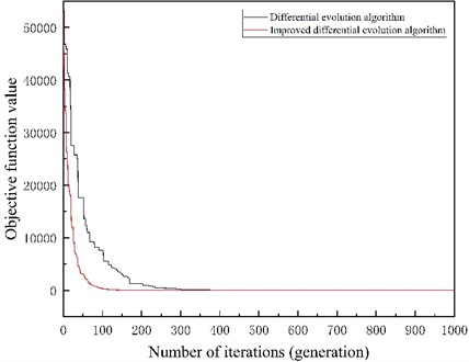
The differential evolutionary algorithm and the modified differential evolutionary algorithm were run the above test functions, each independently for 1000 times before the average value obtained by the two algorithms was obtained by taking the average value of the two algorithms. Among them, the result obtained by the improved differential evolutionary algorithm is 4.64267E-18, and the result obtained by the differential evolutionary algorithm is 0.000894206. The results show that the method by adaptively adjusting the two candidate mutation strategies, the adaptive scaling factor and the crossover rate is an effective improvement scheme to increase the convergence speed and search capability of the algorithm. The modified differential evolutionary algorithm is therefore selected for numerical optimization of the weight matrix in the LQR control of active suspension.

4.3. Adaptation function design

Due to the fact that there are not only unit differences but also different numerical magnitudes between different performance indicators, the design of the fitness function requires de-measurement processing. It is necessary to determine the specific parameters of the vehicle, take the three ride performance evaluation indexes of the passive suspension as the baseline before optimization, and optimize the ratio between the output performance indexes of the LQR controlled suspension and the passive suspension by the improved algorithm as the fitness function of the optimization model. Therefore, the fitness function of the system is designed as follows [23]:

26

m i n L = \frac{B A (X)}{B A_{p}} + \frac{S W S (X)}{S W S_{p}} + \frac{D T D (X)}{D T D_{p}},

X = （q_{1}, q_{2}, q_{3}） 1 0^{- 3} \leq X_{i} \leq 1 0^{7}, （i = 1,2, 3）,

where: $B A$ , $S W S$ , $D T D$ are the corresponding root mean square values of body vertical acceleration, suspension dynamic travel and tire dynamic displacement optimized by the improved algorithm, respectively; ${B A}_{p}$ , ${S W S}_{p}$ , ${D T D}_{p}$ are the three performance indexes of passive suspension, respectively; $X$ is the optimization variable [5].

The optimization of active suspension control necessitates the enhancement of its various performance indicators, specifically ensuring that the root-mean-square value of the optimized output is smaller than the corresponding indicators for passive suspension. In order to guide the population to evolve towards the target direction and find the ideal optimal solution faster, the constraint conditions are designed as:

27

\{\begin{array}{l} B A < B A_{p}, \\ S W S < S W S_{p}, \\ D T D < D T D_{p} . \end{array}

Determine whether each set of weighting coefficients $X$ satisfies Eq. (27), if it does, the fitness function value for that individual is $L$ ; otherwise, to penalize that set of weighting coefficients for not meeting the constraints, take the value of that penalization function $ψ$ to be:

28

ψ = L + 10 .

5. Simulation result analysis

Using MATLAB/Simulink software to build an automobile 1/4 active suspension model and apply LQR control strategy for simulation experiments [24]. The passive suspension, the traditional LQR control of the suspension and the improved differential evolutionary algorithm optimized active suspension LQR control are simulated given the same road inputs [25]. The values of the three performance indicators obtained from the simulation to evaluate the suspension are output. The effectiveness of the improved differential evolutionary algorithm applied to the active suspension LQR control strategy is verified based on the simulation results. The simulation parameters of the active suspension of the vehicle using a certain model are shown in Table 1.

Table 1The main parameters of vehicle simulation

Name	Unit	Numerical value
Sprung mass	kg	40
Unsprung mass	kg	340
Suspension stiffness	N/m	17000
Tire stiffness	N/m	190000
Road roughness coefficient	m3	5×10^-6
Speed of vehicle	m/s	20
Suspension damping stiffness	N·s/m	1400

On the basis of taking the weight coefficient $q_{3} = 1$ of body vertical vibration acceleration, the value of optimization variable $q_{1}$ , $q_{2}$ can be any non-negative value.

After several iterations of optimization, the optimized weight coefficients are obtained by improving the differential evolutionary algorithm as $q_{1} = 104290$ , $q_{2} = 10647$ , $q_{3} =$ 1. The simulation results under different control are analyzed in time domain and frequency domain and compared.

5.1. Time domain analysis

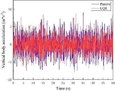
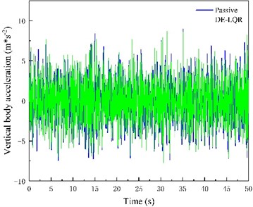
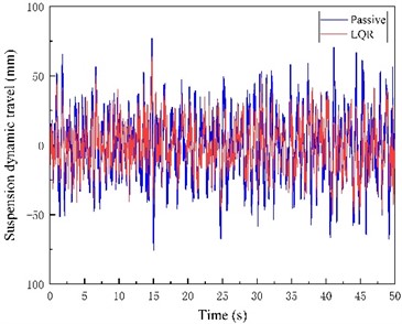
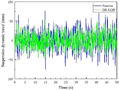
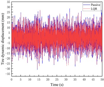
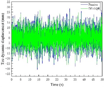
The relevant parameters in the simulation were determined, and the time-domain simulation comparison curves of 3 different performance indicators of the corresponding suspension under different controls were obtained by running the simulation, as shown in Fig. 8. The results of the simulation root-mean-square values were shown in Table 2.

Table 2Comparison of RMS responses of different control time domains

Suspension performance indicators	Uncontrolled	LQR control	LQR control based on improved DE
Vertical body acceleration (m/s²)	2.396	2.375	2.357
Suspension dynamic travel (mm)	23.36	17.11	17.01
Dynamic tire displacement (mm)	7.949	7.639	7.420

Fig. 8Passive Suspension, LQR control suspension, improved differential evolutionary optimization LQR control suspension time domain simulation results

Passive Suspension, LQR control suspension, improved differential evolutionary optimization LQR control suspension time domain simulation results

a)

b)

c)

d)

e)

f)

Fig. 8(a) and (b) include LQR control and modified differential evolution algorithm respectively to optimize the body vertical acceleration diagram of LQR control suspension compared with passive suspension. Fig. 8(c, d) includes the suspension dynamic travel diagram of LQR control and improved differential evolution algorithm to optimize LQR control suspension compared with passive suspension respectively. Fig. 8(e, f) includes the tire dynamic displacement diagram of LQR control and improved differential evolution algorithm to optimize LQR control suspension compared with passive suspension respectively.

Comparison of simulation results between suspension conventional LQR control and suspension LQR control optimized based on improved differential evolutionary algorithm can be seen by inputting the same road excitation. The suspension conventional LQR control optimizes the three performance indexes of BA, SWS, and DTD by 0.8 %, 26.75 %, and 3.80 %, respectively, compared with those of the passive suspension, and the active suspension LQR control optimized based on the improved differential evolution algorithm optimizes the three performance indexes by 1.6 %, 27.1 %, and 6.6 %, respectively, compared with those of the passive suspension.

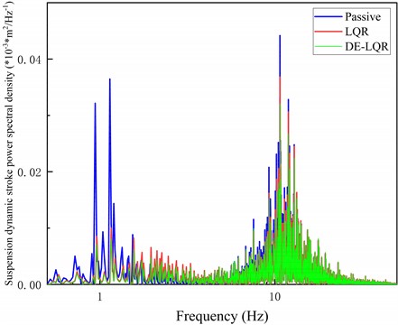
5.2. Frequency domain analysis

The frequency response characteristics of vehicle body, suspension and wheels affect vehicle ride comfort. In order to further analyze and improve differential evolution algorithm to optimize the performance improvement of LQR suspension, frequency domain analysis of various performance indicators of suspension was carried out in MATLAB Simulink, and the analysis results are shown in Figs. 9-11.

In Figs. 9-11, frequency domain analysis is carried out on passive suspension, LQR controlled suspension and LQR controlled suspension optimized by improved differential evolution algorithm respectively. The vertical acceleration, dynamic travel of suspension and peak power spectrum density of tire dynamic displacement of suspension optimized by improved differential evolution algorithm are all reduced to a certain extent compared with LQR controlled suspension. The suspension body vertical acceleration decreased by 19.9 %, the suspension dynamic travel decreased by 1.47 %, and the tire dynamic displacement decreased by 11.2 %.

Fig. 9Comparison of power spectral density of body vertical acceleration under different controls

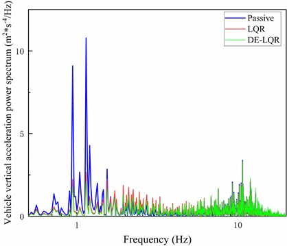
Fig. 10Comparison of dynamic stroke power spectral density of suspension under different controls

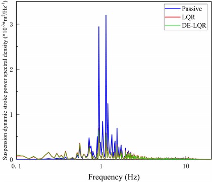
Fig. 11Comparison of tire dynamic displacement power spectral density under different controls

6. Conclusions

In order to overcome the subjective interference of the traditional LQR control in the vehicle active suspension, it is generally necessary to try to put together through the prophet’s experience, and it is easy to appear that it is difficult to obtain the optimal solution for the values of the weighting matrices $Q$ and $R$ . Therefore, the intelligent control algorithm is used to optimize and improve the algorithm, so as to make the LQR controller have a better control effect.

Aiming at the deficiencies, a specific improved differential evolutionary algorithm is proposed, which improves the convergence speed and searching ability and realizes the improvement of the algorithm through the adaptive and self-adaptive adjustment of the scaling factor and crossover rate of the two candidate mutation strategies, and the validity of the improved algorithm is verified by using the test function. This paper builds a 1/4 active suspension simulation model, designs the adaptivity function, and optimizes the value of weight coefficients in the LQR control using the improved differential evolutionary algorithm, so that the LQR controller achieves a more ideal control effect and realizes the fastest speed to solve the global optimal solution of the theory. Simulation studies show that, comparing the simulation results of passive suspension, LQR control suspension, and optimized LQR suspension in the C-class road speed of 20 m/s conditions, it can be seen that the improved differential evolution algorithm has good convergence speed and search ability, which helps to quickly determine the weight matrix, and it is effective to apply it to the active suspension control. Under the time-domain analysis, the LQR control of the traditional suspension makes the BA, SWS, and DTD, which are the 3 performance indexes are optimized by 0.8 %, 26.75 %, and 3.80 %, respectively, compared with those of passive suspension, and the active suspension LQR control optimized based on the improved differential evolutionary algorithm optimizes 1.6 %, 27.1 %, and 6.6%, respectively, compared with the three performance indexes of passive suspension. The peak power spectral density of the frequency domain analysis shows that the improved differential evolutionary algorithm optimized LQR suspension body vertical acceleration is reduced by 19.9 %, suspension dynamic travel is reduced by 1.47 %, and tire dynamic displacement is reduced by 11.2 %. The three performance indexes of the optimized LQR control suspension are all improved to some extent, which ensures the safety of the vehicle and improves the smoothness and ride comfort.

References

P. Amirchoupani, R. Nodeh Farahani, and G. Abdollahzadeh, “The constant damage inelastic displacement ratio for performance design of self-centering systems under far-field earthquake ground motions,” Structures, Vol. 57, p. 105254, Nov. 2023, https://doi.org/10.1016/j.istruc.2023.105254

Publisher
R. Nodeh Farahani, G. Abdollahzadeh, and A. Mirza Goltabar Roshan, “The modified energy-based method for seismic evaluation of structural systems with different hardening ratios and deterioration hysteresis models,” Periodica Polytechnica Civil Engineering, Vol. 68, No. 1, pp. 37–56, Aug. 2023, https://doi.org/10.3311/ppci.21359

Publisher
D. N. Nguyen and T. A. Nguyen, “Evaluate the stability of the vehicle when using the active suspension system with a hydraulic actuator controlled by the OSMC algorithm,” Scientific Reports, Vol. 12, p. 19364, Nov. 2022, https://doi.org/10.1038/s41598-022-24069-w

Publisher
J. Zou, S. Guo, X. Guo, L. Xu, Y. Wu, and Y. Pan, “Hydraulic integrated interconnected regenerative suspension: Modeling and mode-decoupling analysis,” Mechanical Systems and Signal Processing, Vol. 172, p. 108998, Jun. 2022, https://doi.org/10.1016/j.ymssp.2022.108998

Publisher
L. Wu et al., “Vehicle stability analysis under extreme operating conditions based on LQR control,” Sensors, Vol. 22, No. 24, p. 9791, Dec. 2022, https://doi.org/10.3390/s22249791

Publisher
J. Zou, X. Guo, M. A. A. Abdelkareem, L. Xu, and J. Zhang, “Modelling and ride analysis of a hydraulic interconnected suspension based on the hydraulic energy regenerative shock absorbers,” Mechanical Systems and Signal Processing, Vol. 127, pp. 345–369, Jul. 2019, https://doi.org/10.1016/j.ymssp.2019.02.047

Publisher
M. Khamies, G. Magdy, M. Ebeed, and S. Kamel, “A robust PID controller based on linear quadratic gaussian approach for improving frequency stability of power systems considering renewables,” ISA Transactions, Vol. 117, pp. 118–138, Nov. 2021, https://doi.org/10.1016/j.isatra.2021.01.052

Publisher
R. Bai and H.-B. Wang, “Robust optimal control for the vehicle suspension system with uncertainties,” IEEE Transactions on Cybernetics, Vol. 52, No. 9, pp. 9263–9273, Sep. 2022, https://doi.org/10.1109/tcyb.2021.3052816

Publisher
Y. Guo, Y. Wang, K. Meng, and Z. Zhu, “Otsu multi-threshold image segmentation based on adaptive double-mutation differential evolution,” Biomimetics, Vol. 8, No. 5, p. 418, Sep. 2023, https://doi.org/10.3390/biomimetics8050418

Publisher
K. Tashkova, P. Korošec, J. Šilc, L. Todorovski, and S. Džeroski, “Parameter estimation with bio-inspired meta-heuristic optimization: modeling the dynamics of endocytosis,” BMC Systems Biology, Vol. 5, No. 1, p. 159, Jan. 2011, https://doi.org/10.1186/1752-0509-5-159

Publisher
J. Zou, X. Guo, L. Xu, G. Tan, C. Zhang, and J. Zhang, “Design, modeling, and analysis of a novel hydraulic energy-regenerative shock absorber for vehicle suspension,” Shock and Vibration, Vol. 2017, pp. 1–12, Jan. 2017, https://doi.org/10.1155/2017/3186584

Publisher
H. Yan, J. Qiao, S. Zhang, T. Zhao, and Z. Wang, “The optimal control of semi-active suspension based on improved particle swarm optimization,” Mathematical Models in Engineering, Vol. 4, No. 3, pp. 157–163, Sep. 2018, https://doi.org/10.21595/mme.2018.20041

Publisher
H. Yu, C. Zhao, S. Li, Z. Wang, and Y. Zhang, “Pre-work for the birth of driver-less scraper (LHD) in the underground mine: the path tracking control based on an LQR controller and algorithms comparison,” Sensors, Vol. 21, No. 23, p. 7839, Nov. 2021, https://doi.org/10.3390/s21237839

Publisher
J. H. Li, J. He, and X. H. Li, “LQG controller design for heavy vehicle active suspension based on OT-AHP method,” Applied Mechanics and Materials, Vol. 509, pp. 206–212, Feb. 2014, https://doi.org/10.4028/www.scientific.net/amm.509.206

Publisher
L. Wang, P. Jia, T. Huang, S. Duan, J. Yan, and L. Wang, “A novel optimization technique to improve gas recognition by electronic noses based on the enhanced Krill Herd algorithm,” Sensors, Vol. 16, No. 8, p. 1275, Aug. 2016, https://doi.org/10.3390/s16081275

Publisher
L. Liu and R. Zhang, “Multistrategy improved whale optimization algorithm and its application,” Computational Intelligence and Neuroscience, Vol. 2022, pp. 1–16, May 2022, https://doi.org/10.1155/2022/3418269

Publisher
Y. Du, Y. Fan, X. Liu, Y. Luo, J. Tang, and P. Liu, “Multiscale cooperative differential evolution algorithm,” Computational Intelligence and Neuroscience, Vol. 2019, pp. 1–17, Dec. 2019, https://doi.org/10.1155/2019/5259129

Publisher
X. Li et al., “Advanced slime mould algorithm incorporating differential evolution and Powell mechanism for engineering design,” iScience, Vol. 26, No. 10, p. 107736, Oct. 2023, https://doi.org/10.1016/j.isci.2023.107736

Publisher
I. Cruz-Aceves et al., “Multiple active contours guided by differential evolution for medical image segmentation,” Computational and Mathematical Methods in Medicine, Vol. 2013, pp. 1–14, Jan. 2013, https://doi.org/10.1155/2013/190304

Publisher
Y. Deng, T. Zhou, G. Zhao, K. Zhu, Z. Xu, and H. Liu, “Energy saving planner model via differential evolutionary algorithm for bionic palletizing robot,” Sensors, Vol. 22, No. 19, p. 7545, Oct. 2022, https://doi.org/10.3390/s22197545

Publisher
H. M. J. Mustafa, M. Ayob, M. Z. A. Nazri, and G. Kendall, “An improved adaptive memetic differential evolution optimization algorithms for data clustering problems,” Plos One, Vol. 14, No. 5, p. e0216906, May 2019, https://doi.org/10.1371/journal.pone.0216906

Publisher
Y. D. Sergeyev, D. E. Kvasov, and M. S. Mukhametzhanov, “On the efficiency of nature-inspired metaheuristics in expensive global optimization with limited budget,” Scientific Reports, Vol. 8, No. 1, Jan. 2018, https://doi.org/10.1038/s41598-017-18940-4

Publisher
J. Liu, J. Liu, Y. Li, G. Wang, and F. Yang, “Study on multi-mode switching control strategy of active suspension based on road estimation,” Sensors, Vol. 23, No. 6, p. 3310, Mar. 2023, https://doi.org/10.3390/s23063310

Publisher
C. Huang, K. Lv, Q. Xu, and Y. Dai, “Research on the multimode switching control of intelligent suspension based on binocular distance recognition,” World Electric Vehicle Journal, Vol. 14, No. 12, p. 340, Dec. 2023, https://doi.org/10.3390/wevj14120340

Publisher
S. Zhu et al., “Research on stability control algorithm of distributed drive bus under high-speed conditions,” World Electric Vehicle Journal, Vol. 14, No. 12, p. 343, Dec. 2023, https://doi.org/10.3390/wevj14120343

Publisher

About this article

Received

24 January 2024

Accepted

02 May 2024

Published

27 May 2024

SUBJECTS

Vibration in transportation engineering

DOI

https://doi.org/10.21595/jve.2024.23953

Keywords

LQR controller

active suspension

modified differential evolutionary algorithm

Acknowledgements

This research was funded by the Project of National Natural Science Foundation of China (52202480), the Project of Natural Science Foundation of Hubei Province (2022CFB732).

Data Availability

The datasets generated during and/or analyzed during the current study are available from the corresponding author on reasonable request.

Author Contributions

Junyi Zou: model building and writing; Xinkai Zuo: algorithm improvement and grammar checking. All authors have read and agreed to the published version of the manuscript.

Conflict of interest

The authors declare that they have no conflict of interest.

This is an open access article distributed under the Creative Commons Attribution License, which permits unrestricted use, distribution, and reproduction in any medium, provided the original work is properly cited.

Research article

2019 11 28

Effect of in-wheel motor suspension system on electric vehicle ride comfort

Le Van Quynh, Bui Van Cuong, Nguyen Van Liem, Le Xuan Long, Pham Thi Thanh Dung

Research article

2019 08 15

Multi-objective optimization of active suspension predictive control based on improved PSO algorithm

Qiang Zhao, Baoquan Zhu

Research article

2018 12 31

Optimization design of semi-active controller for in-wheel motors suspension

Fangwu Ma, Jiawei Wang, Yang Wang, Longfan Yang

Research article

2018 09 30

The optimal control of semi-active suspension based on improved particle swarm optimization

Haijing Yan, Jubin Qiao, Sen Zhang, Ting Zhao, Zhongchang Wang

J. Zou and X. Zuo, “Active suspension LQR control based on modified differential evolutionary algorithm optimization,” Journal of Vibroengineering, Vol. 26, No. 5, –15, May 2024, https://doi.org/10.21595/jve.2024.23953

Copy Extrica

Copied to clipboard!

TY  - JOUR
DO  - 10.21595/jve.2024.23953
UR  - https://doi.org/10.21595/jve.2024.23953
TI  - Active suspension LQR control based on modified differential evolutionary algorithm optimization
T2  - Journal of Vibroengineering
AU  - Zou, Junyi
AU  - Zuo, Xinkai
PY  - 2024
DA  - 2024/05/27
PB  - Extrica
VL  - 26
IS  - 5
SN  - 1392-8716
SN  - 2538-8460
ER  - 

Copy Ris

Copied to clipboard!

 @article{Zou_2024, title={Active suspension LQR control based on modified differential evolutionary algorithm optimization}, ISSN={2538-8460}, url={https://doi.org/10.21595/jve.2024.23953}, DOI={10.21595/jve.2024.23953}, journal={Journal of Vibroengineering}, publisher={JVE International Ltd.}, author={Zou, Junyi and Zuo, Xinkai}, year={2024}, month=may }

Copy Bibtex

Copied to clipboard!

[1]J. Zou and X. Zuo, “Active suspension LQR control based on modified differential evolutionary algorithm optimization,” Journal of Vibroengineering, May 2024, doi: 10.21595/jve.2024.23953.

Copy IEEE

Copied to clipboard!

Zou, Junyi, and Xinkai Zuo. “Active Suspension LQR Control Based on Modified Differential Evolutionary Algorithm Optimization.” Journal of Vibroengineering, May 27, 2024. https://doi.org/10.21595/jve.2024.23953.

Copy Chicago

Copied to clipboard!

Active suspension LQR control based on modified differential evolutionary algorithm optimization

Abstract

Highlights

1. Introduction

2. Modeling of vehicle control system

2.1. Pavement modeling

2.2. Active suspension modeling

3. LQR controller design

4. Modified differential evolution algorithm and design

4.1. Standard difference evolutionary algorithm

4.2. Differential evolution algorithm optimization strategy

4.3. Adaptation function design

5. Simulation result analysis

5.1. Time domain analysis

5.2. Frequency domain analysis

6. Conclusions

References

About this article

Related Articles