Multi-objective optimization of active suspension predictive control based on improved PSO algorithm

The design and control for active suspension is of great significance for improving the vehicle performance, which requires considering simultaneously three indexes including ride comfort, packaging requirements and road adaptability. To find optimal suspension parameters and provide a better tradeoff among these three performances, this paper presents a novel multi-objective particle swarm optimization (MPSO) algorithm for the suspension design. The mathematical model of quarter-car suspension is first established, and it integrates the hydraulic servo actuator model. Further a model predictive controller is designed for the suspension by using the control strategies of multi-step forecast, rolling optimization and online correction of predictive control theory. To use vehicle body acceleration, tire deflection and suspension stroke to represent the above three performances respectively, a multi-objective optimization model is constructed to optimize the suspension stiffness and damping coefficients. The MPSO algorithm includes extra crossover operations, which are applied to find the Pareto optimal set. The rule to update the Pareto pool is that the newly selected solutions must have two better performances compared with at least one already existed in the Pareto pool, which ensures that each solution is non-dominated within the Pareto set. Finally, numerical simulations on a vehicle-type example are done under B-level road surface excitation. Simulation results show that the optimized suspension can effectively reduce the vertical vibrations and improve the road adaptability. The model predictive controller also shows high robustness with vehicle under null load, half load and full load. Therefore, the proposed MPSO algorithm provides a new valuable reference for the multi-objective optimization of active suspension control.

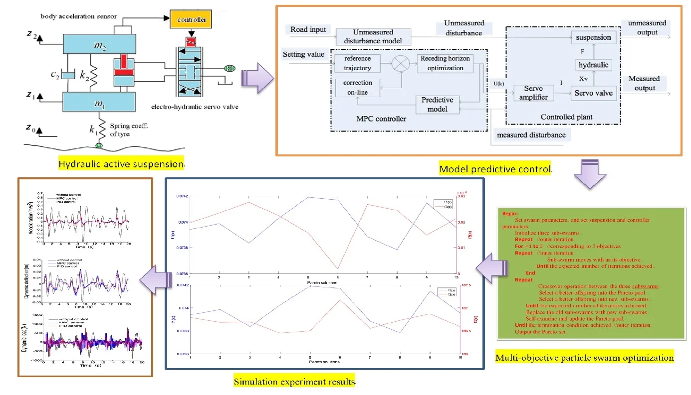
Multi-objective optimization of active suspension predictive control based on improved PSO algorithm

Highlights

Model predictive control (MPC) for hydraulic active suspension.
Novel multi-objective particle swarm optimization (MPSO) algorithm with crossover operations.
Pareto optimization for suspension parameters using MPSO algorithm under MPC.

1. Introduction

Suspension system is one of the crucial parts relative to vehicle ride comfort and road adaptability. A well-designed vehicle suspension is able to isolate the disturbance from road excitation, and meanwhile guarantees better driving smoothness and road adaptability. The traditional passive suspension with fixed-stiffness spring and non-adjustable passive damper is difficult to satisfy the above requirements. The hydraulic active suspension introduces a valve-controlled hydraulic servo cylinder as active actuator parallel to the passive damper and spring. This actuator can present real-time adjustable actuating force according to the vertical acceleration of vehicle body and therefore can greatly improve the performances.

In recent years the study of active suspension has gained the increasing attraction. Fateh and Alavi [1] applied the impedance control in an active vehicle suspension system operated by a hydraulic actuator. Witters and Swevers used a multilayer perception neural network to identify a continuously variable electro-hydraulic semi-active damper for a passenger car and successfully described the complex nonlinear damper dynamics [2]. The skyhook control [3, 4] suits well to improve the comfort but is limited to improve road holding. The linear quadratic control [5] can provide both ride comfort and road holding improvements, but it requires the full state measurement or estimation. The optimal control [6] can provide good performance for the suspension, but it is a well-known fact that the derivation of the control needs the vehicle dynamics to be accurately expressed as a linear model, whereas the vehicle dynamics generally includes nonlinearities and uncertainties. Chen and Huang [7] proposed an adaptive sliding control method for hydraulic active suspension and used function approximation technique to describe the actuator with time-varying uncertainties, further designed a sliding mode control law to make the actuator track the desired skyhook damping asymptotically. Wang and Song et al. [8] used cultural algorithm and niche algorithm to design a Fuzzy-PID controller for active suspension and optimized its fuzzy rules. Besides, backstepping control [9], optimal sliding mode control [10] and robust fault-tolerant control were provided [11, 12].

The method of nonlinear model predictive control (MPC) [13] can be used in different levels of the process control structure and is also able to handle a wide variety of process control constraints systematically. The core idea of predictive control system is to forecast the future output variation trend using the past and the present information. By the method of limited receding horizon optimization, the deviation between the control amount and the target amount should be as small as possible, and the optimization of system control is realized. Literature [14] presented an embedded real-time implementation of the generalized predictive control (GPC) algorithm for automotive active suspension systems and tested it on a hardware-in-the-loop test bench. Literature [15] proposed a new model predictive control algorithm for semi-active air suspension with a multi-mode switchable damper. Up to now, the MPC has been used in the speed tracking control of autonomous ground vehicle [16, 17], lateral stability control and energy management of electric vehicle [18-20]. The above researches all demonstrated the effectiveness of model predictive control, so, in this present study, a nonlinear model predictive controller is designed to improve the performance of hydraulic active suspension.

The design and control of active suspension also involves the key performance indices: ride quality, road adaptability and packaging, and these three terms are represented by sprung-mass acceleration, tire deflection and suspension stroke (also known as the rattle space) respectively. The performance index of vehicle suspension needs to combine these three performance measures using a single objective optimization by assigning adjustable weights to the three performance terms or using the multi-objective optimization based on Pareto solutions. The latter can provide a Pareto set including many Pareto solutions, which ensures the designer to have more options depending on their requirements.

In the last decades, many evolutionary and swarm intelligence algorithms, such as Genetic Algorithm (GA), Ant Colony Optimization (ACO) and Particle Swarm Optimization (PSO) algorithm have been used in the multi-objective optimization domain. As for the suspension optimization without explicit mathematical model and analytic solutions, the above intelligent optimization algorithms show strong power and adaptability, especially the PSO algorithm for its simpler structure and higher computing efficiency. The PSO algorithm is put forward by Kennedy and Eberhart in 1995 [21], and it simulates the food-hunting behavior of bird swarm. The PSO algorithm and its variants have been successfully applied to solve many optimization problems such as intelligent feedback linearization control or fuzzy control of electrohydraulic active and Magnetorheological semi-active suspension systems [22, 23]. Besides some operations of Genetic Algorithm, especially its effective crossover operations, are easily combined with other algorithms [24] to provide us a thought to integrate it into the PSO algorithm to solve the multi-objective optimization problem of active suspension by carrying out further crossover operations among sub-swarms for different optimization objectives.

To solve the tradeoff of the above three performance indexes, this paper employs the Pareto-set based multi-objective optimization to find the optimal suspension parameters which can ensure the suspension with the best performance under the model predictive controller. An improved PSO algorithm with crossover operations is used to solve the multi-objective optimization model, and the Pareto optima are finally obtained.

This paper is organized as follows. The system dynamics of a quarter-car suspension including a hydraulic actuator are derived in Section 2. A model predictive controller is designed in Section 3 using the control strategies of multi-step forecast, rolling optimization and online correction of the predictive control theory. In Section 4, the multi-objective optimization model for the suspension is established, and the improved PSO optimization algorithm is proposed to solve the model. In Section 5, the Simulink model of the hydraulic active suspension with the MPC controller is built, and the optimization program is completed and is run to obtain the Pareto optimal set. The control results of traditional passive mode, PID and the model predictive control are compared under the optimal suspension parameters. Simulations of a vehicle with the operating conditions of null load, half load and full load were done to test the robustness of the MPC controller. Finally, some conclusions are drawn in the last section.

2. Model for active suspension

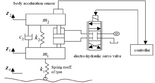
In the active suspension system, an active actuator (hydraulic cylinder) is placed between the sprung mass and unsprung mass parallel to the other suspension elements. Even though this actuator malfunctions, the suspension system can work in the form of passive suspension. The model of quarter car active suspension is shown in Fig. 1. The system consists of two parts of the machinery and hydraulic system. The car body acceleration sensor gets the signal of the car body acceleration and feedbacks it to the controller. The controller figures out the control electric current and sends it to the servo valve. Then the flow of servo valve and the output force of the hydraulic cylinder will be regulated in real time. Therefore, the purpose of attenuating the vehicle body vibration and tire dynamic load can be achieved.

Fig. 1Model of quarter car active suspension

2.1. Dynamics model of suspension

Vehicle suspension system is a very complicated nonlinear system. Based on the modeling process of active suspension, in order to simplify the control model and to extrude the major aspects of research problems, the car body is regarded as a rigid body, and its related parts are taken as linear elements. So, a two DOF model for active suspension is established (Fig. 1). Considering that the tire model is the main factor influencing the optimization result, herein the F-tire (Flexible ring tire model) is selected since it is generally recognized as the preferred tire model for vehicle ride comfort, durability and handling simulation. As shown in Fig. 2(a), the F-tire model includes $C_{r a d}$ , $C_{b e n d}$ , $C_{b e l t}$ , and $C_{t a n g}$ four parts to describe the random bending and to transfer the non-linear stiffness and damping in rotation, longitudinal, lateral direction. In the model, the ride comfort analysis only involves the $C_{r a d}$ part, which includes spring-friction, Maxwell, damper and spring totally four elements to describe the tire radial stiffness with small hysteresis. Herein using the $C_{r a d}$ and the tire experiment loading curve (Fig. 2(b)) to determine the equivalent stiffness value $k_{1}$ of the tire. Based on Newton’s Second Law, the motion equations of the suspension are derived as:

1

\{\begin{array}{l} m_{2} {\ddot{z}}_{2} + c_{2} ({\dot{z}}_{2} - {\dot{z}}_{1}) + k_{2} (z_{2} - z_{1}) - F = 0, \\ m_{1} {\ddot{z}}_{1} + c_{2} ({\dot{z}}_{1} - {\dot{z}}_{2}) + k_{2} (z_{1} - z_{2}) + k_{1} (z_{1} - z_{0}) + F = 0, \end{array}

where $m_{1}$ and $m_{2}$ are the unsprung and the sprung masses, respectively; $c_{2}$ is the average damping coefficient of the dampers; $k_{1}$ is the tire stiffness; $k_{2}$ is the stiffness of the spring connecting the sprung and unsprung masses; $z_{2}$ and $z_{1}$ are the displacements of the sprung and unsprung masses, respectively, and $z_{0}$ is the variation in height of road surface. $F$ is the hydraulic actuation force.

Fig. 2F-tire model

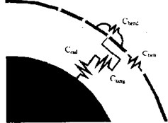
a) Mechanical model

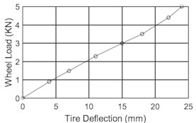
b) Radial characteristic

2.2. Dynamics model of hydraulic actuator

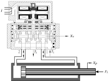
The hydraulic actuator adopts the form of servo valve to control the hydraulic cylinder, the servo valve receives the control electric current and further regulates the hydraulic actuation force, which is a typical servo force system as shown in Fig. 3.

Fig. 3Model of valve controlled hydraulic cylinder

The flow continuity equation of hydraulic cylinder is derived as:

2

Q_{L} = C_{t c} p_{L} + C_{t a} p_{S} + \frac{V_{1}}{β_{e} (1 + η^{3})} {\dot{p}}_{L} + A_{1} {\dot{x}}_{p},

where $p_{s}$ and $p_{L}$ are the supply pressure and the load pressure, respectively; $β_{e}$ is the bulk modulus; $C_{t c}$ and $C_{t a}$ are the total leakage coefficient and system leakage coefficient, respectively; $A_{1}$ and $V_{1}$ are the cross section area and volume of the cylinder, respectively; $η$ is the area ratio of two chambers in the cylinder. $x_{p}$ is the displacement of the hydraulic cylinder piston rod.

The output force equation of hydraulic cylinder piston rod is derived as:

3

F = A_{1} p_{L} = m_{2} {\ddot{x}}_{p} + B_{e} {\dot{x}}_{p} + k x_{p},

where $B_{e}$ is the viscosity damping coefficient; $k$ is the stiffness coefficient of load.

The linear flow equation of servo valve is given as:

4

Q_{L} = K_{q} x_{v} - K_{c} p_{L},

where $K_{q}$ and $K_{c}$ are the servo value flow gain and flow-pressure coefficient, respectively; $x_{v}$ is the displacement of the valve spool.

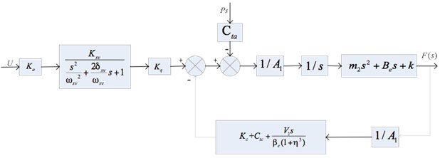
Fig. 4 presents the block diagram of hydraulic actuator according to Eqs. (2), (3) and (4). In this figure, the transfer function of the input current to the valve spool displacement can be simplified as a second order oscillation element:

\frac{X_{v}}{I} = \frac{K_{s v}}{(\frac{s^{2}}{ω_{s v}^{2}} + \frac{2 δ_{s v} s}{ω_{s v}} + 1)},

where $ω_{s v}$ is natural frequency of the servo valve, $δ_{s v}$ is its damping coefficient, and $K_{s v}$ is its gain. The transfer function of the servo amplifier can be simplified as a proportion element: $I$ / $U = K_{a}$ , because its frequency band is much higher than the hydraulic natural frequency.

Fig. 4Block diagram of electro-hydraulic actuator

2.3. Integrated model of suspension system

The dynamics models of suspension and hydraulic actuator are integrated to form the whole system model. First, the state vector is selected as $X = {[z_{1}, z_{2}, {\dot{z}}_{1}, {\dot{z}}_{2}, p_{l}, x_{p}, {\dot{x}}_{p}]}^{T}$ then based on Eqs. (1) to (4), the state-space equations are obtained as:

5

\dot{X} = A X + B U, Y = C X + D U,

where:

A = [\begin{matrix} 0 & 0 & 1 & 0 & 0 & 0 & 0 \\ 0 & 0 & 0 & 1 & 0 & 0 & 0 \\ - \frac{k_{1} + k_{2}}{m_{1}} & \frac{k_{2}}{m_{1}} & - \frac{c_{2}}{m_{1}} & \frac{c_{2}}{m_{1}} & - \frac{A_{1}}{m_{1}} & 0 & 0 \\ \frac{k_{2}}{m_{2}} & - \frac{k_{2}}{m_{2}} & \frac{c_{2}}{m_{2}} & - \frac{c_{2}}{m_{2}} & \frac{A_{1}}{m_{2}} & 0 & 0 \\ 0 & 0 & 0 & 0 & - \frac{β_{e} (1 + η^{3}) （C_{t c} + K_{c}）}{V_{1}} & 0 & - \frac{β_{e} (1 + η^{3}) A_{1}}{V_{1}} \\ 0 & 0 & 0 & 0 & 0 & 0 & 1 \\ 0 & 0 & 0 & 0 & \frac{A_{1}}{m_{2}} & - \frac{k}{m_{2}} & - \frac{B_{e}}{m_{2}} \end{matrix}],

B = [\begin{matrix} 0 & 0 & 0 \\ 0 & 0 & 0 \\ 0 & 0 & \frac{k_{1}}{m_{1}} \\ 0 & 0 & 0 \\ \frac{β_{e} (1 + η^{3}) K_{q}}{V_{1}} & - \frac{β_{e} (1 + η^{3}) C_{t a}}{V_{1}} & 0 \\ 0 & 0 & 0 \\ 0 & 0 & 0 \end{matrix}], C = [\begin{matrix} \frac{k_{2}}{m_{2}} & - \frac{k_{2}}{m_{2}} & \frac{c_{2}}{m_{2}} & - \frac{c_{2}}{m_{2}} & \frac{A_{1}}{m_{2}} & 0 & 0 \\ 1 & - 1 & 0 & 0 & 0 & 0 & 0 \\ - k_{1} & 0 & 0 & 0 & 0 & 0 & 0 \end{matrix}],

D = [\begin{array}{l} 0 & 0 & 0 \\ 0 & 0 & 0 \\ 0 & 0 & k_{1} \end{array}], U = [\begin{array}{l} x_{v} \\ P_{S} \\ z_{0} \end{array}], Y = [\begin{matrix} {\ddot{z}}_{2} \\ z_{1} - z_{2} \\ k_{1} (z_{0} - z_{1}) \end{matrix}] .

The body acceleration, suspension dynamic deflection and tire dynamic load are selected as the output variables. So, in the output vector of $Y$ , ${\ddot{z}}_{2}$ is the body acceleration, $z_{1} - z_{2}$ is the suspension dynamic deflection, and $k_{1}$ ( $z_{0} - z_{1}$ ) is the tire dynamic load.

3. Model predictive control for active suspension system

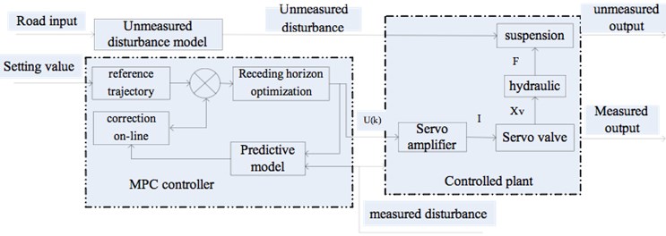
The core idea of model predictive control system is to forecast the future output variation trend using the past and the present information. By the method of limited receding horizon optimization, the deviation between the control amount and the target amount should be as small as possible, and the optimization of system control is realized [13]. The MPC controller for a hydraulic active suspension mainly includes four parts, namely the prediction model, receding horizon optimization, on-line correction and reference trajectory. The structure diagram of the suspension predictive control system is shown in Fig. 5.

Fig. 5Structure diagram of suspension predictive control

3.1. Design of reference trajectory

In the running process of model predictive control, the output will be along a pre-defined curve gradually to approximate the designed expectation, and this curve is the reference trajectory of predictive control. The suspension control belongs to an optimal regulator problem, so the prediction acceleration is defined as zero. Then the system output gradually approaches to zero.

3.2. Design of prediction model

The function of the prediction model is based on the history information of the controlled suspension: ${u (k - j), y (k - j) | j \geq 1}$ and future input: ${u (k + j - 1) | j = 1, \dots, m}$ to forecast the future output ${y (k + j) | j = 1, \dots, p}$ . The predictive control model is discrete, because it uses the receding horizon optimization control. Combining the characteristics of predictive control theory and the real driving conditions, the difference equation can be derived from Eq. (5) [13]:

6

x (k + 1) = A x (k) + B_{u} u (k) + B_{v} v (k) + B_{d} (k),

7

y_{u} (k) = C_{u} x (k) + D_{u u} u (k) + D_{v u} v (k) + D_{d u} d (k),

8

y_{m} (k) = C_{m} x (k) + D_{v m} v (k) + D_{d m} d (k),

where $y_{u} (k) = [k_{1} (z_{0} - z_{1})]^{T}$ is the unmeasured output of system, $y_{m} (k) = [\begin{array}{l} {\ddot{z}}_{2} & z_{1} - z_{2} \end{array}]^{T}$ is the measured output, $u (k) = [x_{v}]^{T}$ is the manipulated variable, $v (k) = [p_{s}]^{T}$ is the measured disturbance, $d (k) = [z_{0}]^{T}$ is the unmeasured disturbance.

3.3. Receding horizon optimization

The purposes of receding horizon optimization is to determine the future manipulated variable through minimizing the performance index, and this index can be described as:

9

J = \sum_{i = 1}^{p} q_{i} (y (k + i) - w (k + i))^{2} + \sum_{j = 1}^{m} r_{j} Δ u^{2} (k + j - 1),

where $Q_{y} = d i a g (\begin{array}{l} q_{1} & q_{2} & \dots & q_{p} \end{array})$ and $R_{u} = d i a g (\begin{array}{l} r_{1} & r_{2} & \dots & r_{m} \end{array})$ , respectively. They are weighting matrices of output variables and manipulated variables. The optimization objective only cares about the dynamic performance of system in the prediction horizon, and it applies the first of the optimal control sequence to the controlled suspension. At time $k$ , the manipulated variable increment is defined as $Δ u (k) = d^{T} (W - Y_{0})$ , in which the variable $d$ may work out ahead of time in an offline way. The new manipulated variable sequence will be obtained by solving the optimization problem after getting a new measurement value in the next sampling moment, and the receding horizon optimization can be realized. The conditions of receding horizon optimization are introduced as below [14]: (1) The mechanical structure of suspension limits its dynamic deflection: $|z_{1} - z_{2}| \leq l_{m a x}$ ; (2) To ensure the tire’s grounding performance, the dynamic load should be less than the static load: $|k_{1} (z_{0} - z_{1})| \leq m g$ ; (3) The engine power restricts the hydraulic actuating force: $|F| \leq F_{m a x}$ .

3.4. On-line correction algorithm

After applying the manipulated variable at moment $k$ , the actual output $y$ ( $k + 1$ ) is not equal to the prediction output of moment $k +$ 1 because of the uncertainty of the suspension parameters and environment. The predictive error is then represented as [13]:

10

e (k + 1) = y (k + 1) - \hat{y} (k + 1) .

This error is weighted and then the prediction output is corrected:

11

{\hat{Y}}_{p} = {\hat{Y}}_{p} + h e (k + 1),

where ${\hat{Y}}_{p} = [\tilde{y} (k + 1), \tilde{y} (k + 2), \dots, \tilde{y} (k + p)]^{T}$ is the predictive output after the error correction at the time $t = (k + 1) T$ , $h = [h_{1}, h_{2}, \dots, h_{p}]^{T}$ is the error correction vector, and $h_{1} =$ 1.

The predictive output ${\hat{Y}}_{p}$ is corrected as the predictive initial value in the next moment. The output of the future moment $t = (k + 2) T, \dots, (k + p + 1) T$ is predicted using the predictive initial value at moment $t = (k + 1) T$ :

12

y_{0} (k + i) = \tilde{y} (k + i + 1), (i = 1,2, \dots, p - 1),

Then the predictive initial value at the next sample moment is expressed as:

13

\{\begin{array}{l} y_{0} (k + i) = \hat{y} (k + i + 1) + h_{i + 1} e (k + 1), \\ y_{0} (k + p) = \hat{y} (k + p) + h_{p} e (k + 1) . \end{array}

The system is transformed into a close-loop negative feedback system because of the introduction of the correction, which plays an important role in improving the system performance.

4. Multi-objective optimization for suspension parameters

4.1. Overview of particle swarm optimization

The PSO algorithm first randomly initializes a swarm of particles. Each particle is represented as $x_{1} = (x_{1}, x_{i, 2}, \dots, x_{i . n})$ , $i = 1,2, \dots, n_{0}$ , where $n_{0}$ is the swarm size, and $n$ is the total dimension number of each particle. Each particle adjusts its trajectory towards its own previous best position $p b e s t_{i}$ , and the previous global best position $g b e s t$ attained by the whole swarm. In the $k$ th iteration, the $i$ th particle with respect to the $j$ th dimension is updated by:

14

v_{i, j}^{(k + 1)} = v_{i, j}^{(k)} + c_{1} r_{1} (p b e s t_{i, j}^{(k)} - x_{i, j}^{(k)}) + c_{2} r_{2} (g b e s t_{j}^{(k)} - x_{i, j}^{(k)}),

15

x_{i, j}^{(k + 1)} = x_{i, j}^{(k)} + v_{i, j}^{(k + 1)},

where $x_{i, j}^{(k)}$ and $v_{i, j}^{(k)}$ are the current position and velocity, respectively. $c_{1}$ and $c_{2}$ are both acceleration constants and generally $c_{1} = c_{2} =$ 2, and $r_{1}$ and $r_{2}$ are both random numbers within the interval of [0, 1].

The procedure of the PSO algorithm for optimization can be described as follows:

(1) Initializing: Generate $n_{0}$ particles with random positions $x_{1}, x_{2}, . . ., x_{n_{0}}$ , and velocities $v_{1}, v_{2}, . . ., v_{n_{0}}$ .

(2) Evaluate the fitness of each particle based on the objective function of the problem.

(3) Individual and global best positions updating: If $f (p b e s t_{i}) > f (x_{i})$ , then let $p b e s t_{i} = x_{i}^{}$ , and search for the minimum value $f_{m i n}$ among $f (p b e s t_{i})$ , If $f (g b e s t) > f_{m i n}$ , let $g b e s t = x_{m i n}$ , $x_{m i n}$ is the particle associated with $f_{m i n}$ .

(4) Velocity updating: update the $i$ th particle velocity using the Eq. (14).

(5) Position updating: update the $i$ th particle position using Eq. (15).

(6) Repeat steps (2) to (5) until the given maximum number of iterations is achieved.

4.2. Multi-objective optimization based on PSO algorithm with crossover operations

The aim of this paper is to find the so-called Pareto optimum (or non-dominated solution). Its definition is as follows:

Definition. A solution $z^{0} \in Z$ is the Pareto optimum for the minimum problem if and only if no other solution $z \in Z$ exists to satisfy [25]:

16

z_{p} < z_{p}^{0}, p \in \{1,2, \dots, q\},

17

z_{l} \leq z_{l}^{0}, p \neq k,

where $Z$ is denoted as the feasible region in the criterion space as:

18

Z = \{z \in R^{q}| z_{1} = f_{1} (x), z_{2} = f_{2} (x), . . ., z_{q} = f_{q} (x), x \in S\},

and $S$ is denoted as the feasible region in the decision space.

To find the Pareto solutions, a new multi-objective PSO algorithm with crossover operations are used as follows. First, three sub-swarms of particles are randomly initialized, and these sub-swarm moves with $f_{i} (x)$ ( $i =$ 1, 2, 3) as its single optimization objective using the above procedure in Section 4.1, respectively. So, after a certain number of iterations, these three sub-swarms revealed some better solutions for each optimization objective respectively. Then the algorithm randomly selects two particles from any two sub-swarms as parent particles and takes the crossover operations between them as follows:

19

{x'}_{i} = α \cdot x_{i} + (1 - α) \cdot x_{j}, x_{j} = (1 - α) \cdot x_{i} + α \cdot x_{j},

where $α$ is a random number extracted from region (0, 1). $x_{i}$ and $x_{j}$ are parent particles. ${x'}_{i}$ and ${x'}_{j}$ are new offspring’s created by crossover operations.

The above crossover operations enable to produce non-dominated Pareto solutions. An additional computing memory called as the Pareto pool is allocated, and it is used to accept and store the Pareto solutions. It is noted that any two offspring’s from crossover operations must be made with mutual comparison before their recruitment into the Pareto pool, and only the dominating one is directly selected into the Pareto pool. If the two offspring’s are non-dominated by each other, one will be selected with the probability into the Pareto set. Further the Pareto pool will also executes self-examination and updating operation in each iteration to remove the newly dominated ones.

4.3. Suspension parameters optimization with MPSO algorithm

For the suspension parameters optimization problem, the decision vector is selected as $x = {x_{i}} = {k_{2}, c_{2}}$ . Considering that there are three performance requirements for the suspension: body acceleration ${\ddot{z}}_{2}$ , suspension dynamic deflection $z_{1} - z_{2}$ and tire dynamic load $k_{1}$ ( $z_{0} - z_{1}$ ), the objective function set is defined as:

20

m i n \{\begin{array}{l} f_{1} (x) = {\ddot{z}}_{2}, & f_{2} (x) = z_{1} - z_{2}, f_{2} (x) = k_{1} (z_{0} - z_{1} \end{array})\},

with three constraints: (1) suspension dynamic deflection $|z_{1} - z_{2}| \leq l_{m a x}$ ; (2) tire dynamic load $|k_{1} (z_{0} - z_{1})| \leq m g$ ; (3) hydraulic actuating force $|F| \leq F_{m a x}$ . Additionally, decision variables also have their range limits as $x_{i, m i n} \leq x_{i} \leq x_{i, m a x}$ , $i =$ 1, 2.

A multi-objective optimization is used to determine the decision vector in order to present the Pareto solutions with the above three performance requirements as the optimization objectives. Based on the above ideas in Section 4.2, the procedure of the multi-objective optimization algorithm is shown in Table 1.

The detailed flowchart of the above optimization algorithm is shown in Fig. 6, whose main program employs the Matlab language (m file) and calls the Simulink model of active suspension controlled by the MPC algorithm.

5. Numerical test

The numerical simulation is completed with the main program written in the Maltab M language, which employs the above optimization algorithm to search the Pareto set and calls the suspension model (with MPC) when evaluating the fitness of each solution. The suspension model with MPC controller is established in Matlab/Simulink as shown in Fig. 7.

The prediction horizon, control horizon and sample time are defined as $P =$ 20, $C =$ 10, and $T =$ 0.002 s. After selecting the constraint limits of input and output, the weighting matrices of manipulated variable and output variable are set respectively. In the Simulink model, the signal type, initial value, simulation time, and so on are selected for the point and disturbance. The simulation parameters setting, referring to the off-road heavy vehicle parameters in literature [26], is shown in Table 2.

Table 1Multi-objective particle swarm optimization algorithm for active suspension

Begin:

Set swarm parameters, and set suspension and controller parameters

Initialize three sub-swarms

Repeat //outer iteration

For

i =

1 to 3 //corresponding to 3 objectives

Repeat //inner iteration

Sub-swarm moves with as its objective

Until the expected number of iterations achieved

End

Repeat

Crossover operation between the three subswarms

Select a better offspring into the Pareto pool

Select a better offspring into new sub-swarms

Until the expected number of iterations achieved

Replace the old sub-swarms with new sub-swarms

Self-examine and update the Pareto pool

Until the termination condition achieved //outer iteration

Output the Pareto set

End

Fig. 6Flowchart of improved PSO algorithm to optimize active suspension with MPC

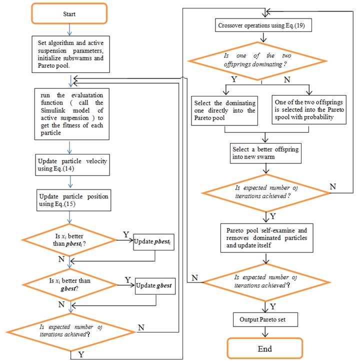
Fig. 7Simulink simulation model

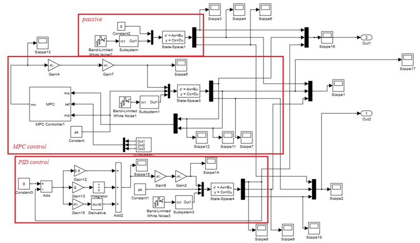
Table 2Simulation parameters

Parameter names	Parameter values	Parameter names	Parameter values
Unsprung mass $m_{1}$ / kg	325	Servo value flow-pressure coefficient $K_{c}$ / m⁵·N^-1·s^-1	2.61×10^-12
Sprung mass $m_{2}$ / kg	1925	Supply pressure $P_{s}$ / Pa	25×10⁶
Tire stiffness coefficient $k_{1}$ / N·m^-1	2.1×10⁵	Load pressure $P_{L}$ / Pa	16×10⁶
Servo value natural frequency $ω_{s v}$ / rad·s^-1	800	Cross section area $A_{1}$ / m²	31.17×10^-4
Damping coefficient $δ_{s v}$	0.6	Cross section volume $V_{1}$ / m³	3.12×10^-4
Servo value gain $K_{s v}$ / M³·S^-1·A^-1	9.82×10^-2	Total leakage coefficient $C_{t c}$ / m⁵·N^-1·s^-1	7.39×10^-13
Viscous damping coefficient $B_{e}$ / N·S·m^-1	4×10⁵	System leakage coefficient $C_{t a}$ / m⁵·N^-1·s^-1	0.01×10^-13
Load stiffness coefficient $k$ / N·m^-1	8×10⁴	Bulk modulus $β_{e}$ / Pa	7×10⁸
Servo value flow gain $K_{q}$	3.2	Area ratio $η$	0.68

Assume the vehicle speed $v =$ 20 m/s, and the road input is a B-level road surface, which is realized with the white noise through a forming filter. the differential of B-level road surface is expressed as ${\dot{x}}_{r} = - 2 π f_{0} x_{r} (t) + 2 π \sqrt{G_{0} v} ω (t),$ where, $x_{r} (t)$ is the road surface vertical displacement, $f_{0}$ is the lower cut-off frequency of road input, $f_{0} =$ 0.01 m^-1, $G_{0}$ is the road roughness coefficient, $ω (t)$ is the band-limited white noise.

The parameters of the MPSO algorithm are set as follows. $n_{0} =$ 20, $n =$ 2, the iteration number of outer iteration is 100, and the inner iteration number is 100. the size of Pareto pool is set as 10. After the simulation is completed, the resultant Pareto set is obtained as shown in Table 3.

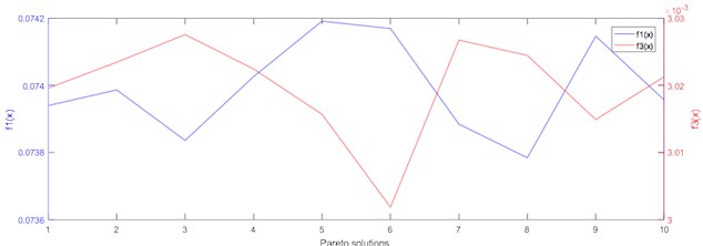
The Pareto frontier is shown in Fig. 8 which describes the Pareto solutions distribution in the 2-D solution space. the 2-D relations of any two of the three objective functions $f_{1} (x)$ , $f_{2} (x)$ and $f_{3} (x)$ are shown in Fig. 9.

Table 3Pareto set and objective functions

No.	Pareto solutions		Objective function values
No.	$x_{1}$	$x_{2}$	$f_{1} (x)$	$f_{2} (x)$	$f_{3} (x)$
1	1.4483493899e+004	2.0344337400e+003	7.3939789709e-002	3.0195903020e-003	1.8679178782e+002
2	1.1597931546e+004	2.2268045635e+003	7.3986498861e-002	3.0234406867e-003	1.8668873656e+002
3	1.1582372225e+004	2.2278418516e+003	7.3836048522e-002	3.0275542613e-003	1.8669886603e+002
4	1.1323563038e+004	2.2450957974e+003	7.4025973644e-002	3.0224399708e-003	1.8644974937e+002
5	1.3484795845e+004	2.1010136103e+003	7.4191307109e-002	3.0156942092e-003	1.8650566772e+002
6	2.1022957177e+004	1.5984695214e+003	7.4169155349e-002	3.0018611568e-003	1.8717702837e+002
7	1.2145038674e+004	2.1903307550e+003	7.3884619974e-002	3.0267336711e-003	1.8655649147e+002
8	1.3866006410e+004	2.0755995726e+003	7.3784280486e-002	3.0244601120e-003	1.8673275366e+002
9	1.3047742023e+004	2.1301505317e+003	7.4146517631e-002	3.0149096846e-003	1.8686995429e+002
10	1.3255734738e+004	2.1162843507e+003	7.3956382200e-002	3.0212819006e-003	1.8659202173e+002

Fig. 8Pareto frontier

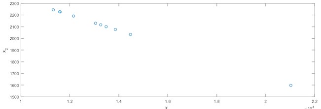
Fig. 9Objective function values of Pareto set

a) $f_{1} (x) - f_{2} (x)$ comparison

b) $f_{1} (x) - f_{3} (x)$ comparison

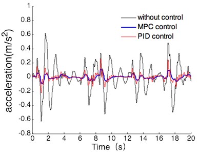
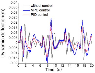
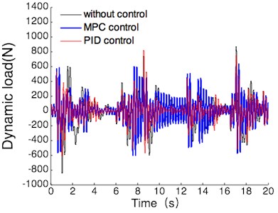
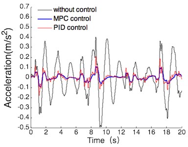
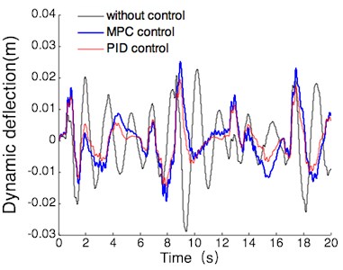
Based on the application conditions and other requirement of suspension, the second solution of the Pareto set is finally selected as the ultimate solution. the performance of the suspension with these optimized parameters is further analyzed. Based on the Simulink model in Fig. 7, the body acceleration, suspension dynamic deflection and tire dynamic load of the suspension under null load, half load and full load conditions are simulated to verify the optimized parameters. the passive mode (without control) and the PID control of the suspension are also completed as the comparison to testify the performance of the MPC control.

(1) With the operating conditions of null load, the simulation results of vehicle body acceleration, suspension dynamic deflection and tire dynamic load are shown in Fig. 10.

Fig. 10Simulation results under null load

a) Vehicle body acceleration

b) Suspension dynamic deflection

c) Tire dynamic load

According to Fig. 10, the simulation comparison results of suspension performance index can be obtained under the operating conditions of null load. the results are shown in Table 4, the values listed in this table are all maxima.

Table 4Suspension performance comparison

Performance index	Acceleration (m/s²)	Dynamic deflection (m)	Dynamic load (N)
Passive	0.62	0.019	866
PID	0.26	0.018	815
MPC	0.11	0.025	629
MPC compared with passive	82 %	–32 %	27 %
MPC compared with PID	58 %	–39 %	23 %

(2) With the operating conditions of half load, the simulation results of vehicle body acceleration, suspension dynamic deflection and tire dynamic load are shown in Fig. 11.

According to Fig. 11, the simulation comparison results of suspension performance index can be obtained under the operating conditions of half load. the results are shown in Table 5, and the values listed in this table are the maxima.

(3) With the operating conditions of full load, the simulation results of vehicle body acceleration, suspension dynamic deflection and tire dynamic load are shown in Fig. 12.

According to the Fig. 12, the simulation comparison results of suspension performance index can be gotten under the operating conditions of full load. the results are shown in Table 6, the values listed in this table are all maxima.

Fig. 11Simulation results under half load

a) Vehicle body acceleration

b) Suspension dynamic deflection

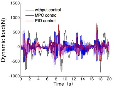
c) Tire dynamic load

Table 5Suspension performance comparison

Performance index	Acceleration (m/s²)	Dynamic deflection (m)	Dynamic load (N)
Passive	0.49	0.029	1065
PID	0.21	0.020	861
MPC	0.11	0.025	640
MPC compared to passive	78 %	14 %	40 %
MPC compared to PID	48 %	–25 %	26 %

Table 6Suspension performance comparison

Performance index	Acceleration (m/s²)	Dynamic deflection (m)	Dynamic load (N)
Passive	0.40	0.032	1142
PID	0.18	0.021	900
MPC	0.11	0.025	670
MPC compared with passive	72 %	22 %	41 %
MPC compared with PID	39 %	–19 %	26 %

From the Tables 4-6 with the operating conditions of null load, half load and full load, the effect of the optimal matching of the main parameters of the tire and suspension on the ride comfort under the model predictive control can be summarized as follows: There are 39 % to 82 % and 23 % to 41 % reductions in the body acceleration and the tire dynamic load compared with those of the passive suspension and the active suspension with PID controller. the suspension dynamic deflection had no notable deterioration compared with that of the passive suspension, and the maximal deflection is still within the permitted range of suspension stroke. The above results mean that the optimized hydraulic active suspension system with a model predictive controller can effectively reduce the vibrations caused by road surface excitation, apparently improved the ride smoothness and road adaptability.

Fig. 12Simulation results full half load

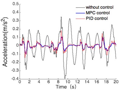
a) Vehicle body acceleration

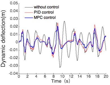
b) Suspension dynamic deflection

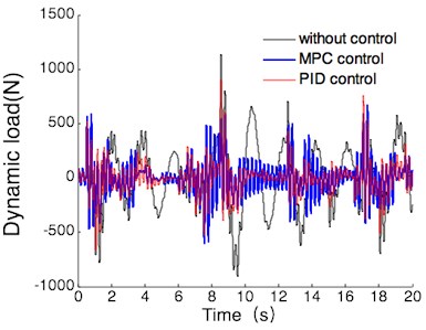
c) Tire dynamic load

6. Conclusions

Based on the active suspension with hydraulic servo actuator, a model predictive controller was designed. the simulation results show that vehicle body acceleration and tire dynamic load were reduced 39 % to 82 % and 23 % to 41 %, and the suspension dynamic deflection had no notable variation as compared with that of the passive suspension with the maximum value of 32 %, with the operating conditions of null load, half load and full load, the optimized active suspension with a model predictive controller can well meet the needs of ride smoothness.

This paper realizes not only the optimal controller by using the MPC but also the optimal suspension parameters by using multi-objective particle swarm optimization algorithm. if the weighted coefficient of input/output, prediction horizon and control horizon of the MPC are optimized, the predictive control effects will be improved in a further study.

References

Fateh M. M., Alavi S. S. Impedance control of an active suspension system. Mechatronics, Vol. 19, 2009, p. 134-140.

Publisher
Witters M., Swevers J. Black-box model identification for a continuously variable, electro-hydraulic semi-active damper. Mechanical Systems and Signal Processing. Mechanical Systems and Signal Processing. Vol. 24, 2010, p. 4-18.

Publisher
Poussot-Vassal C., Sename O., Dugard L., Ramirez-Mendoza R., and Flores L. Optimal skyhook control for semi-active suspensions. Proceedings of the 4th IFAC Symposium on Mechatronics System, Heidelberg, Germany, 2006, p. 608-613.

Publisher
Sammier D., Sename O., Dugard L. Skyhook and H₁ control of active vehicle suspensions: Some practical aspects. Vehicle System Dynamics, Vol. 39, Issue 4, 2003, p. 279-308.

Publisher
Hrovat D. Survey of advanced suspension developments and related optimal control application. Automatica, Vol. 33, Issue 10, 1997, p. 1781-1817.

Publisher
Meditch J. S. Stochastic Optimal Linear Estimation and Control. McGraw-Hill, New York, 1969.

Search CrossRef
Chen P. C., Huang A. C. Adaptive sliding control of active suspension systems with uncertain hydraulic actuator dynamics. Vehicle System Dynamics, Vol. 44, Issue 5, 2006, p. 357-368.

Publisher
Wang W., Song Y. L., Xue Y. B., Jin H. L., Hou J. C., Zhao M. L. an Optimal vibration control strategy for a vehicle’s active suspension based on improved cultural algorithm. Applied Soft Computing, Vol. 28, Issue 1, 2015, p. 167-174.

Publisher
Yagiz N., Hacioglu Y. Backstepping control of a vehicle with active suspensions. Control Engineering Practice, Vol. 16, Issue 6, 2008, p. 1457-1467.

Publisher
Chen S. A., Wang J. C., Yao M., Kim Y. B. Improved optimal sliding mode control for a non-linear vehicle active suspension system. Journal of Sound and Vibration, Vol. 395, Issue 1, 2017, p. 1-25.

Publisher
Van der sande T. P. J., Gysen B. L. J., Besselink L. J. M., Paulides J. J. H., Lomonova E. A., Nijmeijer H. Robust control of an electromagnetic active suspension system: Simulations and measurements. Mechatronics, Vol. 23, Issue 1, 2013, p. 204-212.

Publisher
Wang R. R., Jing H., Karimi H. R., Chen N. Robust fault-tolerant H∞ control of active suspension systems with finite-frequency constraint. Mechanical Systems and Signal Processing, Vols. 62-63, Issues 1, 2015, p. 341-355.

Publisher
Wang L. P. Model Predictive Control System Design and Implementation Using MATLAB. Springer, London, 2009.

Search CrossRef
Shoukry Y., EI-Kharashi M. W., Hammad S. an Embedded implementation of the generalized predictive control algorithm applied to automotive active suspension systems. Computers and Electrical Engineering, Vol. 39, 2013, p. 512-529.

Publisher
Sun X. Q., Yuan C. C., Cai Y.F., Wang S. H., Chen L. Model predictive control of an air suspension system with damping multi-mode switching damper based on hybrid model. Mechanical Systems and Signal Processing, Vol. 94, 2017, p. 94-110.

Publisher
Zhu M., Chen H. Y., Xiong G. M. a Model predictive speed tracking control approach for autonomous ground vehicles. Mechanical Systems and Signal Processing, Vol. 87, 2017, p. 138-152.

Publisher
Besselmann T., Morari M. Hybrid parameter-varying model predictive control for autonomous vehicle steering. European Journal of Control, Vol. 14, Issue 5, 2008, p. 418-431.

Publisher
Xiang C., Ding F., Wang W., He W. Energy management of a dual-mode power-split hybrid electric vehicle based on velocity prediction and nonlinear model predictive control. Applied Energy, Vol. 189, 2017, p. 640-653.

Publisher
Jalali M., Hashemi E., Khajepour A., Chen S. K., Litkouhi B. Integrated model predictive control and velocity estimation of electric vehicles. Mechatronics, Vol. 46, 2017, p. 84-100.

Publisher
Zhang S., Xiong R., Sun F. Model predictive control for power management in a plug-in hybrid electric vehicle with a hybrid energy storage system. Applied Energy, Vol. 185, 2017, p. 1654-1662.

Publisher
Kennedy J., Eberhart R. C. Particle swarm optimization. Proceedings of the 6th IEEE International Conference on Neural Networks, Perth, Australia, 1995, p. 1942-1948.

Search CrossRef
Pedro J., Dangor M., Dahunsi O. A., Ali M. M. Intelligent feedback linearization control of nonlinear electrohydraulic suspension systems using particle swarm optimization. Applied Soft Computing, Vol. 24, 2014, p. 50-62.

Publisher
Talib A., Hussin M., Darus Mat I. Z. Intelligent fuzzy logic with firefly algorithm and particle swarm optimization for semi-active suspension system using magneto-rheological damper. Journal of Vibration and Control, Vol. 23, Issue 3, 2017, p. 501-514.

Publisher
Gao F., Cui G., Liu H. W. Integration of genetic algorithm and cultural algorithms for constrained optimization. International Conference on Neural Information Processing, 2006, p. 817-825.

Publisher
Gen M., Cheng R. W. Genetic Algorithm and Engineering Optimization. John Wiley and Sons, 2000.

Search CrossRef
Yu Y. Parametric simulation of multi-axle off-road vehicle with hydro-pneumatic suspension. Transactions of the Chinese Society for Agricultural Machinery, Vol. 36, Issue 11, 2005, p. 25-28.

Search CrossRef

Cited by

A novel robust adaptive control for nonlinear uncertain quarter-vehicle suspension system in presence of unknown time delay actuation

Samane Fazeli | Alireza Sahab | Ali Moarefianpur

(2024)

2024 International Conference on Telecommunications and Power Electronics (TELEPE)

Taiwu Chen | Zhifu Pan | Guanzhong Xu | Chen Peng | Erjun Liu

(2024)

Research on the Sliding Mode – PID control algorithm tuned by fuzzy method for vehicle active suspension

Tuan Anh Nguyen

(2023)

Research on the Multimode Switching Control of Intelligent Suspension Based on Binocular Distance Recognition

Chen Huang | Kunyan Lv | Qing Xu | Yifan Dai

(2023)

Design a new control algorithm AFSP (Adaptive Fuzzy – Sliding Mode – Proportional – Integral) for automotive suspension system

Tuan Anh Nguyen

(2023)

Analysis of Active Suspension Control Based on Improved Fuzzy Neural Network PID

Mei Li | Jiapeng Li | Guisheng Li | Jie Xu

(2022)

Advance the Efficiency of an Active Suspension System by the Sliding Mode Control Algorithm With Five State Variables

Tuan Anh Nguyen

(2021)

Model Predictive Control of Half-Car Active Suspension Systems Using Particle Swarm Optimisation

Jimoh O. Pedro | Sakhile M.S. Nhlapo | Lindokuhle J. Mpanza

(2020)

About this article

Received

28 December 2017

Accepted

11 December 2018

Published

15 August 2019

SUBJECTS

Vibration in transportation engineering

DOI

https://doi.org/10.21595/jve.2018.19580

Keywords

hydraulic active suspension

multi-objective optimization

model predictive control (MPC)

particle swarm optimization

crossover operations

Acknowledgements

The research work is supported by the Heilongjiang Province Science Foundation (Grant No. LC2015019).

This is an open access article distributed under the Creative Commons Attribution License, which permits unrestricted use, distribution, and reproduction in any medium, provided the original work is properly cited.

Previous article in issue Previous Next article in issue Next

Research article

2021 12 15

PSO optimum control strategy of 7 degrees of freedom semi-active suspensions

Jubin Qiao, Yeonsung Choi, Fuqiang Yang

Research article

2019 09 30

Optimum suspension design for non-linear half vehicle model using particle swarm optimization (PSO) algorithm

Ahmet Yildiz

Research article

2018 11 15

Active control of a nonlinear suspension with output constraints and variable-adaptive-law control

Jun Yao, Jin Qiu Zhang, Ming Mei Zhao, Xin Li

Research article

2018 06 30

Passive fault-tolerant control for vehicle active suspension system based on H2/H∞ approach

Li Ping Zhang, Dong Liang Gong

Q. Zhao and B. Zhu, “Multi-objective optimization of active suspension predictive control based on improved PSO algorithm,” Journal of Vibroengineering, Vol. 21, No. 5, pp. 1388–1404, Aug. 2019, https://doi.org/10.21595/jve.2018.19580

Copy Extrica

Copied to clipboard!

TY  - JOUR
DO  - 10.21595/jve.2018.19580
UR  - https://doi.org/10.21595/jve.2018.19580
TI  - Multi-objective optimization of active suspension predictive control based on improved PSO algorithm
T2  - Journal of Vibroengineering
AU  - Zhao, Qiang
AU  - Zhu, Baoquan
PY  - 2019
DA  - 2019/08/15
PB  - JVE International Ltd.
SP  - 1388-1404
IS  - 5
VL  - 21
SN  - 1392-8716
SN  - 2538-8460
ER  - 

Copy Ris

Copied to clipboard!

@article{Zhao_2019,
	doi = {10.21595/jve.2018.19580},
	url = {https://doi.org/10.21595/jve.2018.19580},
	year = 2019,
	month = {aug},
	publisher = {{JVE} International Ltd.},
	volume = {21},
	number = {5},
	pages = {1388--1404},
	author = {Qiang Zhao and Baoquan Zhu},
	title = {Multi-objective optimization of active suspension predictive control based on improved {PSO} algorithm},
	journal = {Journal of Vibroengineering}
}

Copy Bibtex

Copied to clipboard!

[1]Q. Zhao and B. Zhu, “Multi-objective optimization of active suspension predictive control based on improved PSO algorithm,” Journal of Vibroengineering, vol. 21, no. 5, pp. 1388–1404, Aug. 2019, doi: 10.21595/jve.2018.19580.

Copy IEEE

Copied to clipboard!

Zhao, Qiang, and Baoquan Zhu. “Multi-Objective Optimization of Active Suspension Predictive Control Based on Improved PSO Algorithm.” Journal of Vibroengineering 21, no. 5 (August 15, 2019): 1388–1404. https://doi.org/10.21595/jve.2018.19580.

Copy Chicago

Copied to clipboard!

Multi-objective optimization of active suspension predictive control based on improved PSO algorithm

Abstract

Highlights

1. Introduction

2. Model for active suspension

2.1. Dynamics model of suspension

2.2. Dynamics model of hydraulic actuator

2.3. Integrated model of suspension system

3. Model predictive control for active suspension system

3.1. Design of reference trajectory

3.2. Design of prediction model

3.3. Receding horizon optimization

3.4. On-line correction algorithm

4. Multi-objective optimization for suspension parameters

4.1. Overview of particle swarm optimization

4.2. Multi-objective optimization based on PSO algorithm with crossover operations

4.3. Suspension parameters optimization with MPSO algorithm

5. Numerical test

6. Conclusions

References

Cited by

About this article

Related Articles