Research on active steering control strategy of line-controlled steering system based on MPC

Tong, Yuzhe; Zhang, Xin; Wang, Xinxin; Bai, Yuehong; Yan, Jiao

doi:10.21595/jmeacs.2024.24544

Journal of Mechanical Engineering, Automation and Control Systems

Browse Journal

Submit article

Published: 15 December 2024

Check for updates

Research on active steering control strategy of line-controlled steering system based on MPC

Yuzhe Tong¹

Xin Zhang²

Xinxin Wang³

Yuehong Bai⁴

Jiao Yan⁵

^{1, 2, 3, 4, 5}School of Automotive and transportation, Shenyang Ligong University, Shenyang, China

Corresponding Author:

Xin Zhang

Cite the article Download PDF

Article in Press

Downloads 8

Abstract

In order to improve the stability of the steer by wire (SBW) system during steering, this paper adopts a control strategy based on model predictive control (MPC) to achieve active steering control of the SBW system. Based on the fixed steering gain of the vehicle, design an ideal angular transmission ratio curve, and determine the stability of the vehicle's driving by controlling the yaw rate and center of mass lateral angle, achieving active steering function of the vehicle. Based on Simulink and Carsim platform, establish a vehicle model and analyze the frequency response characteristics of the steering actuator assembly to verify its working stability. The simulation results show that the designed control strategy can significantly improve vehicle handling stability.

1. Introduction

The two main state variables that typically characterize vehicle stability are the center of mass lateral angle and yaw rate. If the deviation between the ideal yaw rate and the actual yaw rate is within a certain range, the vehicle is considered to be in the stable zone, otherwise it is considered to be in the nonlinear zone. When the vehicle becomes unstable, the lateral deviation angle of the center of mass will also rapidly increase. Therefore, it is crucial to keep the vehicle stable in daily life.

References [1-3] adopt the method of keeping the steering gain constant, and design the ideal transmission ratio in segments according to the speed of the vehicle, making it more flexible at low speeds and heavier at high speeds; Reference [4] used H∞ control to effectively track the vehicle's yaw rate; Reference [5] adopts a novel approach rate sliding mode control to effectively improve the stability of wire controlled steering. Reference [6] adopts a fixed time sliding mode control to improve the performance of the steer by wire system. The LQR/LTR method proposed in reference [7] improves the driving stability of vehicles with steer by wire systems. In reference [8], an upper and lower layer control is proposed, and an adaptive sliding control is designed for the upper layer control based on the lateral and yaw angles. In the lower level control, a new adaptive global fast terminal sliding model is proposed. The adaptive part adopts a radial basis function network, which does not require adjustment of system parameters. Verification shows that the hierarchical control performance is superior. Reference [9] designed a fractional-order sliding mode control scheme to address tracking issues and enhance control performance. Additionally, an extended state observer was employed to estimate the aggregated disturbance, with the estimated value then serving as feedforward compensation to mitigate flutter phenomena. Comparative simulation results demonstrate that the proposed SBW control strategy exhibits excellent steering tracking and robust performance.

Hamzah N et al. proposed a sliding mode controller based on wire controlled steering, which can achieve accurate tracking of the response of the reference model for both lateral and yaw movements of four-wheel steering vehicles [10]. Iqbal J et al. estimated the real-time state of the vehicle using a Kalman filter and designed an adaptive global fast sliding mode control to cope with the complex effects of nonlinear factors on the vehicle, while also being able to estimate uncertain system parameters. This scheme has strong robustness and can intelligently adapt to different driving conditions, ensuring that tracking errors can approach zero within a finite time [11]. Mansour Ataei et al. from the University of Waterloo in Canada proposed a new rollover index and used it as the cost function of the MPC algorithm to design an MPC active front wheel steering controller. The experimental results show that the controller can control the car's roll state within a safe range, improving the car's roll stability [12]. Murat Gözü of Istanbul Okan University in Türkiye and others proposed a PI active front wheel steering controller with disturbance observer, in which the disturbance observer is used to observe the internal parameter disturbance of the control system and perform feedforward compensation control. In addition, the controller considers the utilization adhesion coefficient of the inner and outer wheels of the front axle, which improves the lateral stability of the car [13].

The application of the MPC control strategy in this paper can enhance the yaw rate and the sideslip angle of the center of mass, thereby demonstrating the feasibility of this control strategy.

2. Establish a steering control model

2.1. Steer-by-wire system mode

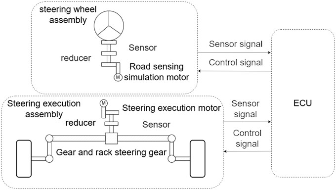
The steer-by-wire system primarily comprises three components the: steering wheel assembly, the main controller, and the steering actuator [14]. The mechanism is shown in Fig. 1. This article mainly studies the four parts of the steering actuator, so it is necessary to establish a dynamic equation for the five mechanisms of the steering motor and gear of the steering actuator.

Fig. 1SBW system structure block diagram

Dynamics equation of steering motor:

1

T_{f m} = J_{f m} {\ddot{θ}}_{f m} + B_{f m} {\dot{θ}}_{f m} + \frac{T_{f s}}{g_{f m}},

2

T_{f s} = K_{f c} (\frac{θ_{f m}}{g_{f m}} - \frac{x_{r}}{r_{p}}),

where $T_{f m}$ is the output torque of the steering motor, that is, the electromagnetic torque; $T_{f s}$ is the torque applied by the motor output to the gear; $B_{f m}$ is the damping constant of the steering motor output shaft; $J_{f m}$ is the moment of inertia of the steering motor; $g_{f m}$ is the reduction ratio of the gearbox for the steering motor; $θ_{f m}$ is the angle of rotation of the output shaft of the steering motor; $r_{p}$ is the radius of the small gear; $X_{r}$ represents the displacement of the gear rack; $K_{f c}$ is the torsional stiffness of the output shaft of the steering motor.

According to Kirchhoff’s second law, the electromotive force balance equation of the motor armature circuit is:

3

U_{f a} = L_{f a} \frac{d i_{f a}}{d t} + R_{f a} i_{f a} + E_{f a},

4

E_{f a} = K_{e 2} {\dot{θ}}_{f m} .

The output torque of the motor shaft is proportional to the armature current:

5

T_{f m} = K_{t 2} i_{f a},

where, $K_{t 2}$ represents the electromagnetic torque constant of the steering motor; $K_{e 2}$ denotes the back electromotive force constant of the steering motor; $E_{f a}$ stands for the back electromotive force of the steering motor; $L_{f a}$ is the inductance of the steering motor; $R_{f a}$ is the resistance of the steering motor; $i_{f a}$ is the current of the steering motor; and $U_{f a}$ is the voltage across the terminals of the steering motor.

Establish the dynamic equation of the gear rack mechanism:

6

\frac{K_{f c}}{r_{p}} (\frac{θ_{f m}}{g_{f m}} - \frac{x_{r}}{r_{p}}) = m_{r} {\ddot{x}}_{r} + B_{r} \dot{x_{r}} + F_{R},

7

F_{R} = \frac{T_{f z l}}{l_{f l}} + \frac{T_{f z r}}{l_{f r}},

where $F_{R}$ is the resistance torque of the rack displacement; $B_{r}$ is the damping cons tant of the rack and pinion; $m_{r}$ is the mass of the rack; $T_{f z l}$ and $T_{f z r}$ are the positive moments of the left and right front wheel cycles, respectively; $L_{f l}$ and $L_{f r}$ are the lengths of the left and right steering knuckles, respectively.

2.2. SBW variable transmission ratio modeling

The ideal transmission ratio adopts a fixed lateral angular velocity gain, and the steady-state transmission ratio formula [3] is:

8

i = \frac{u / L}{G_{δ_{s w}}^{r} (1 + K u^{2})} .

According to the empirical formula, the $G_{δ_{s w}}^{r}$ value of is 0.29, and the formula for obtaining the ideal transmission ratio is:

9

i = f_{i} (u) = \{\begin{array}{l} 7.2, u \leq 20 k m / h, \\ \frac{u / L}{0.29 (1 + K u^{2})}, 20 k m / h \leq u \leq 100 k m / h, \\ 22.8, u \geq 100 k m / h . \end{array}

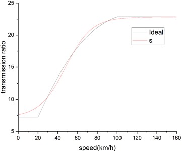
When the vehicle is near the critical speed, the angular acceleration of the motor suddenly changes back and forth, resulting in unstable output torque of the motor and excessive energy loss. Therefore, it is necessary to handle the ideal transmission ratio and use an improved s-function [15] fitting to make it smoother. The fitting formula is:

10

f_{s} (\begin{matrix} u \end{matrix}) = i_{m i n} + \frac{i_{m a x} - i_{m i n}}{1 + e^{- ε (\begin{matrix} u - τ \end{matrix})}},

where $τ$ and $ε$ are both adjustment coefficients, and the proximity coefficient $ζ$ represents the degree of closeness of the fitting curve. 160 is the upper limit of the vehicle speed. According to its calculation formula, the adjustment coefficient under the best fitting effect can be obtained:

11

ξ = \int_{0}^{160} [f_{s} (u) - f_{i} (u)]^{2} d u .

Fig. 2 shows the modified ideal transmission ratio, which serves as the variable angle transmission ratio for the SBW system.

Fig. 2modified ideal transmission ratio

3. Design of vehicle stability control strategy

3.1. Linear 2 DOF model

According to the linear 2 DOF Model [16], the ideal center of mass sideslip angle and yaw rate can be calculated, and the two degree of freedom model is crucial for the design of stability controllers:

12

\{\begin{matrix} m v_{x} (\dot{β} + γ) = - 2 C_{f} (δ - β - \frac{l_{f} γ}{v_{x}}) - 2 C_{r} (\frac{l_{r} γ}{v_{x}} - β), \\ I_{z} \dot{γ} = - 2 C_{f} l_{f} (δ - β - \frac{l_{f} γ}{v_{x}}) + 2 C_{r} l_{r} (\frac{l_{r} γ}{v_{x}} - β), \end{matrix}

where $∆ δ$ represents the additional angle of AFS, and $δ = δ_{f} + ∆ δ$ , signifying that the total angle is the adjustment of the AFS additional angle to the front wheel angle; $C_{f}$ and $C_{r}$ denote the lateral stiffness of the vehicle’s front and rear tires, respectively.

Transform into state space form:

13

\{\begin{array}{l} {\dot{x}}_{t} = A_{t} x_{t} + B_{u} δ_{f} + B_{u} u_{t}, \\ y_{t} = C_{t} x_{t}, \end{array}

where $x_{t} = {[β, γ]}^{T}$ , $u_{t} = {[Δ δ]}^{T}$ , $y = {[β, γ]}^{T}$ , $β$ is the lateral deviation angle of the center of mass, $γ$ is the yaw rate, and $δ_{f}$ is the front wheel steering angle:

A_{t} = [\begin{matrix} \frac{2 C_{f} + 2 C_{r}}{m v_{x}} & \frac{2 l_{r} C_{r} - 2 l_{f} C_{f}}{m v_{x}^{2}} - 1 \\ - \frac{2 l_{f} C_{f} - 2 l_{r} C_{r}}{I_{z}} & - \frac{2 l_{f}^{2} C_{f} + 2 l_{r}^{2} C_{r}}{I_{z} v_{x}} \end{matrix}] = [\begin{matrix} a_{11} & a_{12} \\ a_{21} & a_{22} \end{matrix}],

B_{u} = [\begin{matrix} \frac{2 C_{f}}{m v_{x}} \\ \frac{2 l_{f} C_{f}}{I_{z}} \end{matrix}] = [\begin{matrix} b_{1} \\ b_{2} \end{matrix}], C = [\begin{matrix} 1 & 0 \\ 0 & 1 \end{matrix}] .

Finally, the formula is discretized using the forward Euler method to obtain the following formula:

14

x (k + 1) = A (k) x (k) + B_{u} (k) u (k) + B_{u} (k) δ_{f} (k),

y (k) = C (k) x (k) .

The forward Euler method is to decompose the state variables into $\dot{x} = \frac{x (k + 1) - x (k)}{T}$ simplified ones through term shifting. From this, it can be concluded that:

15

I = [\begin{matrix} 1 & 0 \\ 0 & 1 \end{matrix}], A (\begin{matrix} k \end{matrix}) = A_{t} T + I, B (\begin{matrix} k \end{matrix}) = B_{u} T, C (\begin{matrix} k \end{matrix}) = C .

3.2. Control strategy based on yaw rate and sideslip angle

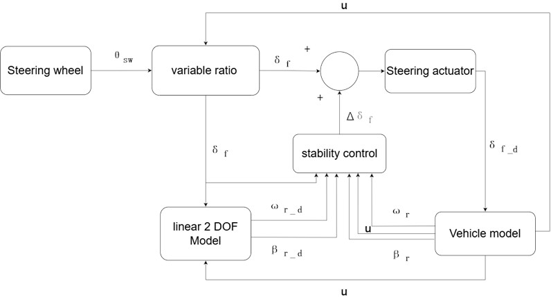
Utilizing a control strategy centered on yaw rate and sideslip angle, this paper integrates a holistic control approach for both variables to implement a multi-input single-output system, achieving more pronounced control effects than those of a single-input single-output system. The active steering control strategy of the steer-by-wire system is illustrated in Fig. 3. The system calculates the front-wheel angle based on the steering wheel angle and longitudinal velocity, then inputs these values into a two-degree-of-freedom model to derive the desired yaw rate and center of mass lateral angle. On one hand, Model Predictive Control (MPC) projects the dynamic model to forecast the center of mass lateral angle and yaw rate for the forthcoming n steps. It computes errors by subtracting the actual states from the desired states for these n steps and then accumulates these errors to minimize the overall discrepancy. On the other hand, the strategy aims to reduce the front-wheel turning angle as much as possible, with both components forming the basis of the cost function. Ultimately, the supplementary front-wheel steering angle is determined through quadratic programming, which is then implemented by the steering actuator to direct the wheels.

3.3. Model predictive control strategy design

Based on the formula for the Linear 2 DOF Model, it follows that when $\dot{β} = 0$ , $\dot{γ} = 0$ , the vehicle is in a steady state, at which point the center of mass’s side slip angle and yaw rate will be constant and stable. Simultaneous equations for solution:

16

\{\begin{matrix} \dot{β} = 0, \\ \dot{γ} = 0 . \end{matrix}

By substituting $\dot{x} = {[0, 0]}^{T}$ into Eq. (13), the steady-state center of mass lateral angle and yaw rate can be simplified and defined as:

17

\{\begin{matrix} β_{s} = \frac{(a_{12} b_{2} - a_{22} b_{1})}{(a_{11} a_{22} - a_{12} a_{21})} \cdot δ_{f}, \\ γ_{s} = \frac{(a_{21} b_{1} - a_{11} b_{2})}{(a_{11} a_{22} - a_{12} a_{21})} \cdot δ_{f}, \end{matrix}

where $a_{i j} (i, j = 1,2)$ , $b_{i} (i = 1,2)$ are shown in Eq. (13).

Fig. 3Integrated control block diagram for active steering

The yaw rate $β$ and the center of mass lateral angle $γ$ are important parameters for measuring vehicle stability. Under normal circumstances, when the vehicle's center of mass sideslip angle is small, the stability can be described by the yaw rate. However, when the vehicle deviates significantly from the trajectory, that is, when the center of mass sideslip angle is large, the yaw rate cannot accurately characterize the vehicle's stable state. The yaw rate and center of mass lateral angle for a typical vehicle are:

18

\{\begin{array}{l} β_{s s} = \min \{|β_{s}|, |\arctan (0.02 μ g)|\} sgn (β_{s}), \\ γ_{s s} = \min \{|γ_{s}|, |\frac{0.85 μ g}{ν_{x}}|\} sgn (γ_{s}) . \end{array}

Change Eq. (14) to an incremental model, to eliminate static errors:

19

Δ x (k + 1) = x (k + 1) - x (k) = A (k) Δ x (k) + B_{u} (k) Δ u (k) + B_{u} (k) Δ δ_{f} (k),

y (k) = C (k) Δ x (k) + y (k - 1),

where $Δ x (k) = x (k) - x (k - 1)$ , $Δ u (k) = u (k) - u (k - 1)$ , $Δ δ_{f} (k) = δ_{f} (k) - δ_{f} (k - 1)$ .

To derive the predictive model, it is necessary to assume that the front wheel steering angle difference input by the driver in the control time domain remains unchanged:

Δ δ_{f} (k) = Δ δ_{f} (k + 1) = Δ δ_{f} (k + 2) = Δ δ_{f} (k + 3) = . . . = Δ δ_{f} (k + m) .

Perform prediction deduction:

\begin{matrix} Δ x (k + 2 | k) = A Δ x (k + 1 | k) + B_{u} Δ u (k + 1) + B_{u} Δ δ_{f} (k + 1) \\ = A^{2} Δ x (k) + A B_{u} Δ δ_{f} (k) + A B_{u} Δ u (k) + B_{u} Δ u (k + 1), \\ ︙ \\ Δ x (k + N c | k) = A^{N c} Δ x (k) + A^{N c - 1} B_{u} Δ δ_{f} (k) + A^{N c - 1} B_{u} Δ u (k) \\ + A^{N c - 2} B_{u} Δ u (k + 1) + \dots + B_{u} Δ u (k + N c - 1), \\ ︙ \\ Δ x (k + N p | k) = A^{N p} Δ x (k) + A^{N p - 1} B_{u} Δ δ_{f} (k) + A^{N p - 1} B_{u} Δ u (k) \\ + A^{N p - 2} B_{u} Δ u (k + 1) + \dots + A^{N p - N c} B_{u} Δ u (k + N c - 1), \end{matrix}

where $Δ x (k + N p | k)$ represents the state prediction of the $k$ -th time for the $k + N p$ -th time Substitute into the output of Eq. (19):

\begin{matrix} y (k + 2 | k) = C A Δ x (k + 1 | k) + C B_{u} Δ u (k + 1) + C B_{u} Δ δ_{f} (k + 1) \\ = C A^{2} Δ x (k) + C A B_{u} Δ u (k) + C B_{u} Δ u (k + 1) + C B_{u} Δ δ_{f} (k), \\ ︙ \\ y (k + N c | k) = C A^{N c} Δ x (k) + C A^{N p - 1} B_{u} Δ δ_{f} (k) + C A^{N c - 1} B_{u} Δ u (k) \\ + C A^{N c - 2} B_{u} Δ u (k + 1) + \dots + C B_{u} Δ u (k + N c - 1), \\ ︙ \\ y (k + N p | k) = C A^{N p} Δ x (k) + C A^{N p - 1} B_{u} Δ δ_{f} (k) + C A^{N p - 1} B_{u} Δ u (k) \\ + C A^{N p - 2} B_{u} Δ u (k + 1) + \dots + C A^{N p - N c} B_{u} Δ u (k + N c - 1) . \end{matrix}

Write the above equation in matrix form:

20

Y_{p} (k + 1 | k) = S_{x} Δ x (k) + I y (k) + S_{u} Δ U (k) + S_{d} Δ δ_{f} (k) .

Where predict the time domain as $N p$ and control the time domain as $N c$ :

Y_{p} (k + 1| k) = [\begin{matrix} y (k + 1| k) \\ y (k + 2| k) \\ ⋮ \\ y (k + N p| k) \end{matrix}], Δ U (k) = [\begin{matrix} Δ u (k) \\ Δ u (k + 1) \\ ⋮ \\ Δ u (k + N c - 1) \end{matrix}],

S_{x} = [\begin{matrix} C A \\ \overset{2}{\sum_{i = 1}} C A^{i} \\ ⋮ \\ \overset{N p}{\sum_{i = 1}} C A^{i} \end{matrix}], I = [\begin{matrix} I_{n_{y} \times n_{y}} \\ I_{n_{y} \times n_{y}} \\ ⋮ \\ I_{n_{y} \times n_{y}} \end{matrix}], S_{d} = [\begin{matrix} C A B_{u} \\ \overset{2}{\sum_{i = 1}} C A^{i} B_{u} \\ ⋮ \\ \overset{N p}{\sum_{i = 1}} C A^{i} B_{u} \end{matrix}],

\begin{array}{l} S_{u} = [\begin{matrix} C B_{u} & 0 & 0 & \dots & 0 \\ \overset{2}{\sum_{i = 1}} C A^{i - 1} B_{u} & C B_{u} & 0 & \dots & 0 \\ ⋮ & ⋮ & ⋮ & ⋱ & ⋮ \\ \overset{N c}{\sum_{i = 1}} C A^{i - 1} B_{u} & \overset{N c - 1}{\sum_{i = 1}} C A^{i - 1} B_{u} & \dots & \dots & C B_{u} \\ ⋮ & ⋮ & ⋮ & ⋱ & ⋮ \\ \overset{N p}{\sum_{i = 1}} C A^{i - 1} B_{u} & \overset{N p - 1}{\sum_{i = 1}} C A^{i - 1} B_{u} & \dots & \dots & \overset{N p - N c + 1}{\sum_{i = 1}} C A^{i - 1} B_{u} \end{matrix}] . \end{array}

List the cost function, the purpose of designing the cost function is to obtain the optimal control sequence. Find $H$ and $f$ :

21

J = {∥Y_{p} - R_{r e f}∥}_{Q}^{2} + {∥Δ U∥}_{R}^{2} + {∥ε∥}_{ρ}^{2} = {(S_{x} Δ x (k) + I y (k) + S_{u} Δ U (k) + S_{d} Δ δ_{f} (k) - R_{r e f})}^{T} Q (S_{x} Δ x (k) + I y (k) + S_{u} Δ U (k) + S_{d} {Δ δ}_{f} (k) - R_{r e f}) + Δ U {(k)}^{T} R Δ U (k) + ε^{T} ρ ε = {[\begin{matrix} Δ U (k) \\ ε \end{matrix}]}^{a} [\begin{matrix} S_{u}^{T} Q S_{u} + R & 0 \\ 0 & ρ \end{matrix}] [\begin{matrix} Δ U (k) \\ ε \end{matrix}] + [\begin{matrix} 2 (S_{x} Δ x (k) + I y (k) + S_{d} {Δ δ}_{f} (k) - R_{r e f}) Q S_{u} & 0 \end{matrix}] [\begin{matrix} Δ U (k) \\ ε \end{matrix}] = \frac{1}{2} X^{T} H X + f X,

where $ρ$ represents the weight of the soft constraint, it is designed to prevent unsolvable situations. If the first two terms of $J$ cannot be solved, the solver can reduce the gradient of the third soft constraint to obtain a solution with looser constraints. The coefficient is typically set to 10. $R_{r e f}$ is a vector composed of expected values. Subsequently, when addressing the constraints, to ensure the control law and its growth constraints are met at each prediction time, the control laws for subsequent prediction times must be cumulatively applied:

\begin{array}{l} U (k + 1) = Δ U (k + 1) + U (k), \\ U (\begin{matrix} k + 2 \end{matrix}) = Δ U (\begin{matrix} k + 2 \end{matrix}) + Δ U (\begin{matrix} k + 1 \end{matrix}) + U (\begin{matrix} k \end{matrix}), \\ ⋮ \\ U (\begin{matrix} k + N p \end{matrix}) = Δ U (\begin{matrix} k + N p \end{matrix}) + \dots + Δ U (\begin{matrix} k + 1 \end{matrix}) + U (\begin{matrix} k \end{matrix}) . \end{array}

Write it in matrix form:

\begin{array}{l} I u_{m i n} \leq U \leq I u_{m a x}, \\ I u_{m i n} \leq A_{I} Δ U + U (k) \leq I u_{m a x}, \\ I u_{m i n} - U (k) \leq A_{I} Δ U \leq I u_{m a x} - U (k) . \end{array}

At the same time, constraints must be added to each increment of the control law to ensure that the growth rate of the control law for each operation is within a certain range. This constraint is treated as upper and lower limits in QP solving:

22

Δ u_{m i n} \leq Δ U (k) \leq Δ u_{m a x},

where $Δ u_{m i n} = [\begin{array}{l} - 0.0082 \end{array}]$ , $Δ u_{m a x} = [\begin{array}{l} 0.0082 \end{array}]$ , $u_{m i n} = [\begin{array}{l} - 0.54 \end{array}]$ , $u_{m a x} = [\begin{array}{l} 0.54 \end{array}]$ . Due to the presence of soft constraints, the last value of the output quantity is the soft constraint $ε$ , which is limited to the range of 0 to 10. So the upper and lower limits of the final output are constrained as follows:

23

l b = [\begin{matrix} Δ u_{m i n}; 0 \end{matrix}],

u b = [\begin{matrix} Δ u_{m a x}; M \end{matrix}] .

Finally, quadratic programming is performed using quadprog to obtain the corresponding incremental additional rotation angle. Then, the current additional rotation angle is obtained by combining the incremental additional rotation angle with the previous one:

24

u_{r e a l} (k) = Δ u (k) + u_{l a s t} (k) .

Then add the driver’s front wheel steering angle to obtain the final steering angle:

25

u_{m p c} = u_{r e a l} + δ_{f} .

4. Simulation analysis

To validate the accuracy of the developed model and control strategy, this study employs sine wave and double lane change maneuvers for simulation. The road adhesion coefficient is set to 0.2, the speed to 60 km/h, and the simulation lasts for 15 seconds. The results of the double lane change maneuver are depicted in the subsequent figure.

Fig. 4Lateral displacement curve

As illustrated in Fig. 4, among the uncontrolled, variable transmission ratio control, and MPC control, the lateral peak value under MPC control is 3.99 m, representing a 4.1 % decrease from the uncontrolled model. Consequently, the MPC control strategy effectively enhances trajectory tracking capability, thereby increasing vehicle stability.

Fig. 5Yaw rate curve

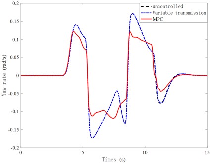
As shown in Fig. 5 under MPC control, the peak yaw rate is the lowest, and the response is relatively smooth compared to the uncontrolled and variable transmission ratio control. Compared with the uncontrolled model, the peak value decreases by 29.4 %. Simulation shows that this control strategy can effectively regulate the vehicle’s yaw rate, ensuring good stability.

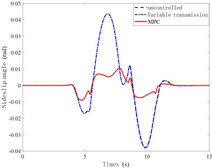
As shown in Fig. 6, this control strategy can minimize the variation Sideslip angele and significantly reduce the peak value, achieving a 75 % reduction compared to the uncontrolled state. Simulations demonstrate that the MPC control strategy can notably enhance the lateral stability at medium speeds and low adhesion conditions, thereby ensuring that the SBW system can travel along a normal trajectory and exhibit excellent trajectory tracking capabilities.

Fig. 6Sideslip angele curve

The road adhesion coefficient is set to 0.85, with a simulation time of 15 seconds and a speed of 80 Km/h. The simulation results under sinusoidal conditions are shown in the following figure.

Fig. 7Yaw rate curve

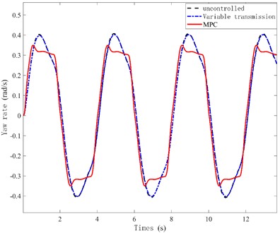
Fig. 8Sideslip angele curve

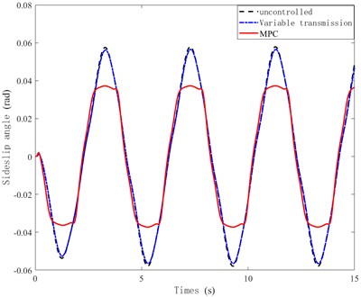
Fig. 7 shows that under MPC control, the peak yaw rate is the lowest, and the response is relatively gentle compared to uncontrolled and variable transmission ratio control. Compared with the uncontrolled model, the peak value decreases by 12.3 %. Simulation shows that this control strategy can effectively adjust the yaw rate of the vehicle, ensuring good stability.

From Fig. 8, it is evident that this control strategy leads to a smaller change in the sideslip angele and a notable reduction in peak value, with a decrease of 35.4 % compared to the uncontrolled state. Simulation results indicate that MPC can significantly enhance the lateral stability of high-speed and high-adhesion conditions, thereby ensuring that the SBW system can travel and maintain stability along normal trajectories.

5. Conclusions

This study develops a Model Predictive Control (MPC) system with soft constraints, establishing a control strategy that integrates feedback from yaw rate and sideslip angele, significantly enhancing the vehicle's handling and stability. Through tests on a medium-speed, low-adhesion road surface featuring double lane changes, and high-speed, high-adhesion sinusoidal maneuvers, it was observed that the vehicle's center of sideslip angele and yaw rate were effectively suppressed under the integrated control, aligning more closely with ideal values, thereby demonstrating the strategy's effective performance. Throughout the tests, the vehicle's response speed and control precision met the anticipated outcomes, confirming the feasibility and advantage of the designed MPC control strategy for practical applications. Further analysis indicates that this control strategy not only effectively manages complex driving scenarios but also maintains stable control across various road conditions, offering reliable technical support for enhancing the dynamic capabilities of smart vehicles. The control strategy outlined in this study shows substantial benefits in improving vehicle safety and controllability.

References

H. Zheng, S. Ma, and X. Na, “Design of a variable steering ratio for steer-by-wire vehicle with a joystick,” Advances in Mechanical Engineering, Vol. 9, No. 11, p. 168781401773075, Nov. 2017, https://doi.org/10.1177/1687814017730753

Publisher
H. Zheng, C. Zong, C. Tian, and Etc, “Automobile steer by wire control algorithm based on ideal steering transmission ratio,” Journal of Jilin University (Engineering Edition), Vol. 2007, No. 6, pp. 1229–1235, 2007, https://doi.org/10.13229/j.cnki.jdxbgxb2007.06.018

Publisher
Wan Weijie, “Research on active steering control strategy of front wheel wire controlled steering system,” Hunan University, 2022.

Search CrossRef
F. Xu, C. Zhou, J. Wang, and Etc, “Research on extensible H ∞ control method for all wheel steer by wire vehicles based on variable transmission ratio,” Chinese Journal of Highways, Vol. 34, No. 9, pp. 133–145, 2021, https://doi.org/10.19721/j.cnki.1001-7372.2021.09.011

Publisher
H. Huang, Y. Gao, W. Wang, and Etc, “Sliding mode control of intelligent unmanned vehicle steer by wire system based on a new approach law,” Journal of Beijing Institute of Technology, Vol. 43, No. 8, pp. 773–782, 2023, https://doi.org/10.15918/j.tbit1001-0645.2022.172

Publisher
P. Gongyu and L. Siqing, “Fixed time sliding mode control of wire controlled steering system with fault-tolerant performance,” Journal of Chongqing University of Technology (Natural Sciences), Vol. 37, No. 6, pp. 48–57, 2023.

Search CrossRef
H. Zhang and W. Z. Zhao, “Stability control strategy of steer-by-wire system based on LQG/LTR,” Science China Technological Sciences, Vol. 60, pp. 844–853, 2017.

Publisher
L. Chen and L. Tang, “Yaw stability control for steer-by-wire vehicle based on radial basis network and terminal sliding mode theory,” Proceedings of the Institution of Mechanical Engineers, Part D: Journal of Automobile Engineering, Vol. 237, No. 8, pp. 2036–2048, 2023.

Publisher
Q. Shi et al., “Extended state observer based fractional order sliding mode control for steer‐by‐wire systems,” in IET Control Theory and Applications, 2023.

Publisher
N. Hamzah et al., “Yaw stability improvement for four wheel active steering vehicle using sliding mode control,” in IEEE 8th International Colloquium on Signal Processing and its Applications, 2012.

Publisher
J. Iqbal, K. Zuhaib, C. Han, A. Khan, and M. Ali, “Adaptive global fast sliding mode control for steer-by-wire system road vehicles,” Applied Sciences, Vol. 7, No. 7, p. 738, Jul. 2017, https://doi.org/10.3390/app7070738

Publisher
M. Ataei, A. Khajepour, and S. Jeon, “Model predictive rollover prevention for steer-by-wire vehicles with a new rollover index,” International Journal of Control, Vol. 93, No. 1, pp. 140–155, 2020.

Publisher
M. Gözü, B. Ozkan, and M. T. Emirler, “Disturbance observer based active independent front steering control for improving vehicle yaw stability and tire utilization,” International Journal of Automotive Technology, Vol. 23, No. 3, pp. 841–854, 2022.

Publisher
G. Cong, “Simulation of road feeling and transmission ratio characteristics of wire controlled steering,” Hefei University of Technology, Hefei, 2017.

Search CrossRef
B. Zhou, L. Fan, and X. Lv, “Design of improved variable transmission ratio curve for active front wheel steering system,” China Mechanical Engineering, Vol. 25, No. 20, pp. 2813–2818, 2014.

Search CrossRef
X. Ma, P. K. Wong, and J. Zhao, “Cornering stability control for vehicles with active front steering system using TS fuzzy based sliding mode control strategy,” Mechanical Systems and Signal Processing, Vol. 125, pp. 347–364, 2019.

Publisher

About this article

Received

13 September 2024

Accepted

13 November 2024

Published

15 December 2024

DOI

https://doi.org/10.21595/jmeacs.2024.24544

Keywords

variable angle transmission ratio

active steering

vehicle stability

MPC

Acknowledgements

This research was funded by Basic Research Funds for Undergraduate Universities in Liaoning Province (Project No. SYLUGXTD07).

Data Availability

The datasets generated during and/or analyzed during the current study are available from the corresponding author on reasonable request.

Author Contributions

Yuzhe Tong: model building, data curation, software, original draft preparation and editing. Xin Zhang: manuscript review, put forward comments, and provide methodological ideas. Xinxin Wang: manuscript review. Jiao Yan: original draft preparation and editing.

Conflict of interest

The authors declare that they have no conflict of interest.

This is an open access article distributed under the Creative Commons Attribution License, which permits unrestricted use, distribution, and reproduction in any medium, provided the original work is properly cited.

Research article

2020 06 29

Road handling improvement through active yaw control system using feedforward sliding mode controller

Vijayapragas Muniandy, Kevin Ong

Research article

2019 08 15

Multi-objective optimization of active suspension predictive control based on improved PSO algorithm

Qiang Zhao, Baoquan Zhu

Research article

2019 03 31

Integrated yaw and rollover stability control of an off-road vehicle with mechanical elastic wheel

Haiqing Li, Youqun Zhao, Fen Lin, Han Xu

Research article

2017 06 30

Hybrid model predictive control of damping multi-mode switching damper for vehicle suspensions

Xiaoqiang Sun, Yingfeng Cai, Chaochun Yuan, Long Chen, Ruochen Wang

Y. Tong, X. Zhang, X. Wang, Y. Bai, and J. Yan, “Research on active steering control strategy of line-controlled steering system based on MPC,” Journal of Mechanical Engineering, Automation and Control Systems, Vol. 5, No. 2, –12, Dec. 2024, https://doi.org/10.21595/jmeacs.2024.24544

Copy Extrica

Copied to clipboard!

TY  - JOUR
DO  - 10.21595/jmeacs.2024.24544
UR  - https://doi.org/10.21595/jmeacs.2024.24544
TI  - Research on active steering control strategy of line-controlled steering system based on MPC
T2  - Journal of Mechanical Engineering, Automation and Control Systems
AU  - Tong, Yuzhe
AU  - Zhang, Xin
AU  - Wang, Xinxin
AU  - Bai, Yuehong
AU  - Yan, Jiao
PY  - 2024
DA  - 2024/12/15
PB  - Extrica
VL  - 5
IS  - 2
SN  - 2669-2600
SN  - 2669-1361
ER  - 

Copy Ris

Copied to clipboard!

 @article{Tong_2024, title={Research on active steering control strategy of line-controlled steering system based on MPC}, ISSN={2669-1361}, url={https://doi.org/10.21595/jmeacs.2024.24544}, DOI={10.21595/jmeacs.2024.24544}, journal={Journal of Mechanical Engineering, Automation and Control Systems}, publisher={JVE International Ltd.}, author={Tong, Yuzhe and Zhang, Xin and Wang, Xinxin and Bai, Yuehong and Yan, Jiao}, year={2024}, month=dec }

Copy Bibtex

Copied to clipboard!

[1]Y. Tong, X. Zhang, X. Wang, Y. Bai, and J. Yan, “Research on active steering control strategy of line-controlled steering system based on MPC,” Journal of Mechanical Engineering, Automation and Control Systems, Dec. 2024, doi: 10.21595/jmeacs.2024.24544.

Copy IEEE

Copied to clipboard!

Tong, Yuzhe, Xin Zhang, Xinxin Wang, Yuehong Bai, and Jiao Yan. “Research on Active Steering Control Strategy of Line-Controlled Steering System Based on MPC.” Journal of Mechanical Engineering, Automation and Control Systems, December 15, 2024. https://doi.org/10.21595/jmeacs.2024.24544.

Copy Chicago

Copied to clipboard!

Research on active steering control strategy of line-controlled steering system based on MPC

Abstract

1. Introduction

2. Establish a steering control model

2.1. Steer-by-wire system mode

2.2. SBW variable transmission ratio modeling

3. Design of vehicle stability control strategy

3.1. Linear 2 DOF model

3.2. Control strategy based on yaw rate and sideslip angle

3.3. Model predictive control strategy design

4. Simulation analysis

5. Conclusions

References

About this article

Related Articles