Abstract
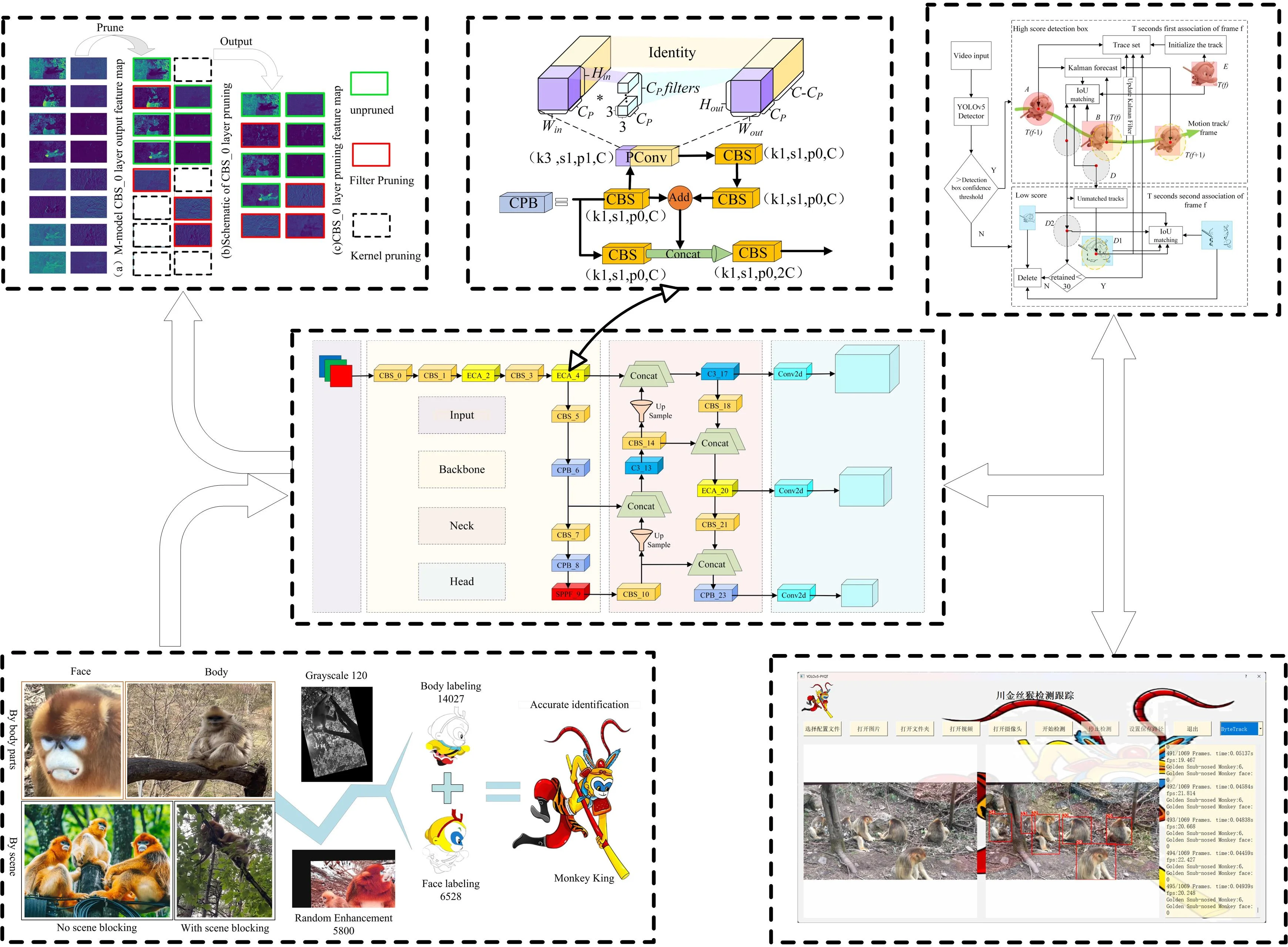
To enable rapid detection of golden snub-nosed monkeys in complex environments, reduce the human costs associated with tracking and observing these monkeys, and accelerate the development of intelligent forest monitoring, we propose the PCB-YOLOv5n-prune model. This model is designed for lightweight devices and is based on channel pruning and module reconstruction. First, we constructed a dataset that combines annotations of the golden snub-nosed monkey's face and body, with some data converted to grayscale. We mixed and expanded five data styles to decrease reliance on color and enhance the informational content. Next, we applied the Sparse Group Lasso selection operator method to slim down the YOLOv5n primitive model for golden snub-nosed monkey detection, improving the detection speed of the underlying network. We then introduced a lightweight convolutional module, PConv, to create the improved residual branching module, CPB, which reduces model computation and memory access. Additionally, we incorporated a lightweight attention module, ECA, to adaptively weight channel features, facilitating local cross-channel information interaction. Finally, we integrated the ByteTrack multi-target tracking algorithm to enable continuous tracking of golden snub-nosed monkeys and visualize detection results. Experimental results demonstrate that the PCB-YOLOv5n-prune model reduces the number of parameters, floating point operations, and model weight by 61 %, 56 %, and 55 %, respectively, compared to the original YOLOv5n model, while significantly improving detection speed.
Highlights
- First, we constructed a dataset that combines annotations of the golden snub-nosed monkey's face and body, with some data converted to grayscale. We mixed and expanded five data styles to decrease reliance on color and enhance the informational content.
- Next, we applied the Sparse Group Lasso selection operator method to slim down the YOLOv5n primitive model for golden snub-nosed monkey detection, improving the detection speed of the underlying network.
- We then introduced a lightweight convolutional module, PConv, to create the improved residual branching module, CPB, which reduces model computation and memory access.
- Additionally, we incorporated a lightweight attention module, ECA, to adaptively weight channel features, facilitating local cross-channel information interaction.
- Finally, we integrated the ByteTrack multi-target tracking algorithm to enable continuous tracking of golden snub-nosed monkeys and visualize detection results.
1. Introduction
The golden snub-nosed monkey (Rhinopithecus roxellanae) [1], is a unique protected species in China, often referred to as the “Monkey King” due to its striking appearance, and is beloved by the Chinese people. Its population development plays a crucial role in maintaining the stability of forest ecosystems and holds significant academic research value [2-3]. However, the survival and reproduction of golden snub-nosed monkeys face serious threats and challenges due to the over-exploitation of natural resources and climate change [4]. To enhance the protection of this species and preserve biodiversity, observation and research on golden snub-nosed monkeys have become particularly important.
The rapid development of computer vision has enabled the use of lightweight devices combined with target detection algorithms as an alternative to manual inspection for intelligent monitoring of golden snub-nosed monkey habitats. However, this approach places high demands on the real-time performance and deployment capabilities of the detection algorithms [5-6]. As a result, lightweight detection algorithms with lower hardware performance requirements have become crucial for the intelligent monitoring of golden snub-nosed monkeys.
In recent years, the detection and recognition of golden snub-nosed monkeys have entered an intelligent phase due to the incorporation of convolutional neural networks (CNNs). Fang Nan et al. [7] applied residual convolution to the CNN model to enhance the feature fusion capabilities of the network layers, effectively recognizing the faces of golden snub-nosed monkeys. Wang Gewei et al. [8] utilized a Self-Paced Learning strategy to optimize the training process of Bilinear Convolutional Neural Networks, helping to avoid local optima. Hu Xu et al. [9] improved the convolutional neural network model AKP-CNN (Attention Key Part Convolutional Neural Network) by integrating attention mechanisms, allowing for the separate extraction of global and local features, and achieving focused fusion of key feature regions .These studies primarily focus on facial recognition of golden snub-nosed monkeys, which makes it challenging to meet the detection needs of these monkeys in the wild when relying solely on facial information. To address this, Sun Rui et al. [10] combined facial features with body features and achieved individual detection of golden snub-nosed monkeys in the field through parameter optimization of Faster R-CNN [11], demonstrating effective detection across various scenarios. Faster R-CNN is classified as a two-stage detection algorithm, which generally offers better detection accuracy; however, it falls short in real-time detection performance. In contrast, single-stage detection algorithms directly predict the category and location of targets using dense networks and anchor frames [12]. These algorithms feature smaller models, faster detection speeds, and are more suitable for real-time applications. Among these, YOLOv5 is particularly popular due to its straightforward structure. Mathew et al. [13] proposed a method using the YOLOv5 model to detect bacterial spot disease in bell pepper plants from photographs taken in the farm, aiming to prevent the spread of plant diseases. Meanwhile, Puliti et al. [14] utilized the largest model in the YOLOv5 series, YOLOv5x, to classify the extent of snow breakage in trees. Zhang Fan et al. [15] reconfigured the YOLOv5s backbone network using MBConvBlock and constructed the ECBAM module to enhance network performance while reducing the number of parameters, achieving effective detection of the crested ibis. Sun Han et al. [16] employed a Shuffle block as a lightweight module to replace the YOLOv5 backbone, compressing the model’s volume by 39.4 % while effectively extracting features from a distance. Yang Wenhan et al. [17] enhanced YOLOv5s by using a weighted channel splicing method in conjunction with the Swin Transformer module and CNN, improving feature extraction and fusion capabilities, particularly for small target animals. Overall, YOLOv5 demonstrates high maturity and practicality in the field of target detection.
To address the limitations of existing golden snub-nosed monkey detection algorithms, which exhibit weak real-time performance and low deployment efficiency, this paper proposes a detection algorithm based on YOLOv5n. The approach includes designing a model pruning process to lighten the front-end model, applying the Sparse Group Lasso selection operator method [18] to achieve channel sparsity in the model, and simultaneously developing a lightweight module called CPB. Additionally, the ECA [19] attention mechanism is incorporated to reconstruct the model. This results in a significant reduction in computational complexity while maintaining detection accuracy, thereby providing technical support for the intelligent monitoring of golden snub-nosed monkeys.
2. Data sets and methods
2.1. Production of data sets
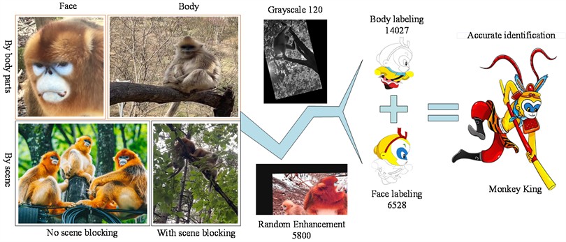
The dataset used in this experiment consists of self-media footage from Foping Panda Valley (33°40'6.183"N, 107°58'23.92"E) in Shaanxi Province. To increase the diversity of the background, web crawling was also performed on golden snub-nosed monkeys from different habitats, resulting in a total of 2,872 data images. Unclear target images were removed, yielding 1,040 valid images. 120 randomly selected images were converted to three-channel grayscale images to reduce dependence on target color. Given that the faces of golden snub-nosed monkeys are often small targets and facial features are prone to occlusion, leading to missed detections, body data was also included as a detection feature. The Labelimg annotation tool was used to annotate the faces and bodies of golden snub-nosed monkeys in the constructed 1,160 images in YOLO format, forming the initial dataset. The dataset is divided according to the body parts of golden snub-nosed monkeys into facial data and trunk data; and according to the target scene into data with scene occlusion and data without scene occlusion, with scene occlusion further divided into background occlusion and target-to-target occlusion. As shown in Fig. 1.
By applying random flips, random brightness adjustments, random saturation changes, random pixel shifts, and the addition of salt-and-pepper noise to the initial dataset, the total number of images was increased to 5,800. This augmented dataset includes 14,027 body targets and 6,528 monkey face targets (Fig. 1). A random seed of 123 was set for the augmented dataset, which was then divided into training, validation, and test sets in an 8:1:1 ratio.
Fig. 1Sample data sets and processing
2.2. Overall technical approach
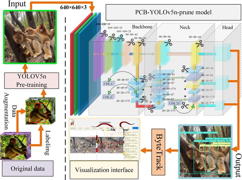
The overall process of the golden snub-nosed monkey detection algorithm is outlined in this paper, as shown in Fig. 2. After completing the labeling and division of the augmented dataset, it is fed into the YOLOv5n network. Using transfer learning methods, general features are extracted from a large dataset to obtain a generalized pre-trained model. Redundant parameters are pruned and detection performance is enhanced through channel pruning and network reconstruction, resulting in the PCB-YOLOv5 prune model. The detection boxes output by the model are combined with the ByteTrack [20] target tracking algorithm to achieve continuous tracking and visualization of multiple golden snub-nosed monkeys.
2.2.1. YOLOv5n pruning algorithm based on sparse group Lasso
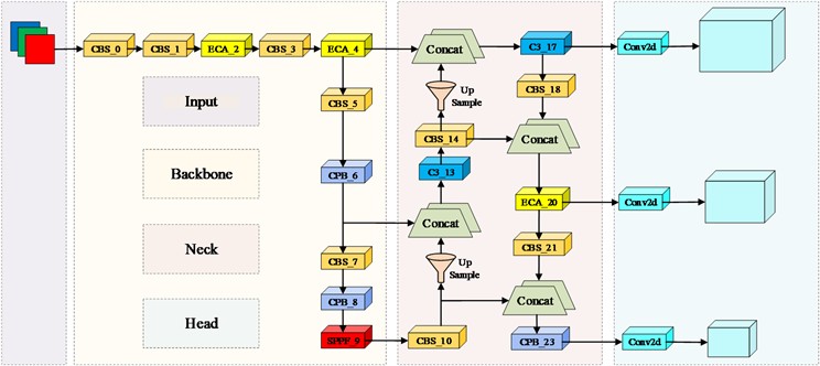
YOLOv5n features a simple structure and fast detection speed, making it particularly suitable for targets that move quickly, have fewer categories, and possess simple features. Therefore, the model selected for detecting golden snub-nosed monkeys uses a depth multiplier of 0.33 and a width multiplier of 0.25 as the base model. The model can be divided into four parts: Input, Backbone, Neck, and Head. The Input section is responsible for data processing and anchor box calculations, the Backbone section is tasked with feature extraction, the Neck section handles multi-scale feature fusion, and the Head section, in conjunction with weighted Non-Maximum Suppression (NMS), outputs the optimal detection boxes for regression prediction.
The divided dataset was then input into the network for training. The fine-tuned YOLOv5n can detect golden snub-nosed monkeys with high precision, but the model has a large number of redundant parameters. To simplify the model’s complexity and improve detection efficiency, a channel pruning algorithm is used to prune the sparsified YOLOv5n.
Fig. 2Overall process overview
The parameters of the Batch Normalization (BN) layer in YOLOv5n are used as the predictive factor for slimming the network, allowing us to assess the importance of each channel. One advantage of this approach is that it does not introduce additional computations to the network. We employ a multi-task penalty (Sparse Group Lasso) algorithm to induce sparsity at both the group and individual feature levels, facilitating the selection of predictive factors both within and across groups. The loss function is given by Eqs. (1-3):
where, and represent the input and output values during network training, respectively, while denotes the weight parameters in the training process. and are the regularization balancing factors that control the sparsity within and between groups, respectively. is the set of predictive factors, and is the number of feature groups, derived from the grouping information of prior variables. This loss function sums the absolute values of each coefficient while also aggregating the L2 norms of the coefficients within each group. During the optimization process, this structure aims to achieve inter-group sparsity; however, the constraints for intra-group sparsity are not sufficiently strong. Therefore, by applying L1 norm penalties to the absolute values of the coefficients, a sparse solution is provided to compensate for the intra-group constraints.
2.2.2. Design of CPB lightweight module
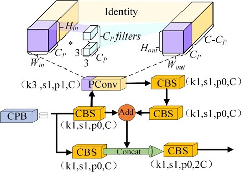
To avoid the loss of critical information caused by extensive pruning, this paper employs a model reconstruction approach prior to pruning for parameter optimization. The C3 module of YOLOv5n incorporates partial convolution modules (PConv), as shown in Fig. 3, with a kernel size set to 3×3. Additionally, the original Bottleneck branch, which uses a 3×3 kernel size CBS, is replaced with two CBS layers that use 1×1 kernels to form a PB (PConv-Bottleneck) residual branch. The number of branches is set to a multiple of 3, corresponding to the product of the model’s depth multiplier. After tensor concatenation of the PB branch with the CBS using a 1×1 kernel, it is fed into another CBS with a 1×1 kernel to achieve a change in channel dimensions, forming the CPB module. In this setup, PConv applies CBS for spatial feature extraction on CP input channels, where the input equals the output for this part of the convolution, while the remaining channels output through an identity mapping, maintaining an input and output channel count of C. A classic ratio of CP:C=1:4 is used, and the formulas for the FLOPs and MAC (Memory Access Cost) of the convolution layer, excluding bias terms, are shown in Eq. (4) and Eq. (5):
The computational cost of PConv is 1/16 that of CBS, which is consistent with the test results:
The memory access volume of PConv is approximately 1/4 that of CBS. This reduction leads to a decrease in the overall parameter computation of the CPB module, lowers memory access frequency, and has a minimal impact on feature extraction performance.
Fig. 3CPB module structure Diagram
2.2.3. Introduction of the ECA attention module
During neural network training, attention mechanisms are often incorporated to optimize the network model. This mechanism works by autonomously learning to reduce the learning weights of less important parts of the input data while enhancing the weights of more significant parts. To improve the accuracy of the pruned model, this experiment employs Efficient Channel Attention (ECA), which assigns weights to each channel. This is achieved by introducing a learnable 1D convolution layer that captures the dependencies between channels. The convolution layer performs global average pooling on the feature maps of each channel to provide a global description of the channels. The ECA module adaptively determines the kernel size based on the number of channels , as shown in Eq. (6):
where, the parameters and are hyperparameters of the ECA attention mechanism. The parameter is used to adjust the attention weights, while the parameter is used to shift the attention weights. The value of is obtained by taking the absolute value and rounding down to the nearest odd number , ensuring that the kernel size is odd.
Once the kernel size is determined, the ECA module applies a one-dimensional convolution to the input features, allowing it to learn the importance of each channel relative to the others. This process can be represented by the following Eq. (7):
where, represents a one-dimensional convolution operation with a kernel size of , denotes the channel, and represents the Sigmoid activation function. As the number of channels increases, the range of local cross-channel interactions also expands. The ECA attention module achieves performance improvements without significantly increasing the computational burden.
The improved model PCB-YOLOv5n obtained from the aforementioned YOLOv5n model is shown in Fig. 4.
Fig. 4Improved network mode
2.2.4. Combining ByteTrack for tracking golden snub-nosed monkeys
Combining the improved YOLOv5n with the IoU-based ByteTrack algorithm, we estimate the trajectories of multiple moving targets and assign unique identity identifiers (IDs). The video is transmitted to the improved YOLOv5 to generate target detection boxes. Based on a confidence threshold, the detection boxes are classified into high-confidence and low-confidence boxes. The ByteTrack algorithm performs the following operations based on the detection box conditions, as shown in Fig. 5.
Fig. 5ByteTrack algorithm diagram
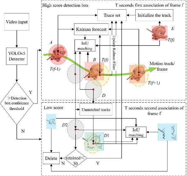
Using Kalman filtering, the position information A of the target trajectory at frame is predicted to obtain the predicted position of the target trajectory at frame . The predicted position information of the -frame trajectory is associated with the target position information of frame using IoU to calculate distance and similarity metrics, and the Hungarian algorithm is employed for matching. For the successfully matched trajectory set B, the Kalman filter is updated, and the trajectories are added to the trajectory collection, while the high-confidence detection boxes that were not matched to any trajectory are retained in collection E, along with the trajectory collection D that has not matched any detection boxes.
Next, the unmatched trajectory collection D is assessed against the low-confidence detection boxes using a second IoU similarity measurement. For the successfully matched trajectory collection D1, the Kalman filter is updated, and the trajectories are added to the trajectory collection. Low-confidence detection boxes that fail to match can be considered background and are directly removed.
The unmatched high-confidence detection boxes in collection E may represent newly appeared targets, and they are initialized as new inactive trajectories. In the next frame cycle, it is checked whether there are any detection boxes that match, which will determine if they are activated. For the trajectories in collection D2 that fail to match a second time, they are retained for 30 frames before being deleted and are included in the trajectory prediction for frame .
This process is repeated to achieve ID tracking of multiple targets.
2.3. Experimental platform and evaluation criteria
2.3.1. Experimental platform
The experiment was conducted on the Ubuntu 20.04.5 LTS operating system, with a processor model of Intel(R) Core(TM) i7-6800K CPU @ 3.40GHz×12 and a graphics card model of NVIDIA CORPORATION GP102[TITAN Xp]. The deep learning framework used was PyTorch 1.21 with CUDA 11.3, the programming platform was PyCharm, and the programming language was Python 3.8. All algorithm comparisons were performed in the same environment. To improve model training efficiency, custom parameters were set: the image input size was set to 640×640 pixels, the learning rate was set to 0.009, the number of data loading processes was set to 4, and the batch size was set to 16 to fully utilize the GPU. After multiple preliminary experiments, the training epoch was set to 200.
2.3.2. Evaluation criteria
To comprehensively evaluate the model’s performance, the experiment utilized several computational performance metrics, including the number of parameters (Params) or model weight and floating point operations (FLOPs). Additionally, recognition performance metrics included the mean Average Precision (mAP), Precision (P), and Recall (R) to assess the effectiveness of the experimental model. The recognition performance metrics involve True Positives (TP), False Negatives (FN), False Positives (FP), and True Negatives (TN). Based on TP, FN, FP, and TN, the formulas for Precision P and Recall R are shown in Eqs. (8-9):
Mean Average Precision (mAP) is the average of Average Precision (AP) for two categories (the face and body of the golden snub-nosed monkey). AP measures the average precision of a model for a single class. A higher mAP value indicates better detection performance of the model. The calculation of AP and mAP is shown in Eqs. (10-11):
where represents the number of categories. To improve the detection of golden snub-nosed monkeys, this study averages the detection accuracies of the monkey’s face and body to derive the final detection accuracy. The purpose of this approach is to learn richer features from these two categories and reduce the miss rate caused by partial target omission.
3. Experiment and analysis
3.1. Pruning results and analysis
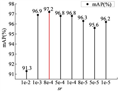
Sparsity training selects channels by setting different sparsity rates (). If the value is too small, the sparsity process becomes too slow, and the effect of weights approaching zero is not significant, making it difficult to distinguish the importance of channels. Conversely, if the value is too large, it may set the weights of important channels to zero, often resulting in a rapid decline in accuracy. To determine the optimal sparsity rate, multiple experiments with different sparsity rates were conducted, setting the values to 1e-2, 1e-3, 8e-4, 5e-4, 1e-4, 8e-5, 5e-5, and 1e-5, followed by sparsity training on YOLOv5n. Fig. 6 illustrates the trend of coefficient changes corresponding to different sparsity rates. It can be observed that as training progresses, the coefficients gradually approach zero, and the higher the sparsity rate, the faster the coefficients approach zero. After sparsity training, all models underwent 50 % pruning, and Fig. 7 compares the parameters of the pruned models. It is evident that when the sparsity rate is 8e-4, the pruned model achieves the highest mAP. Therefore, this study selects a sparsity rate of 8e-4.
Fig. 6BN layer γ coefficient under different sparsity rates (sr)
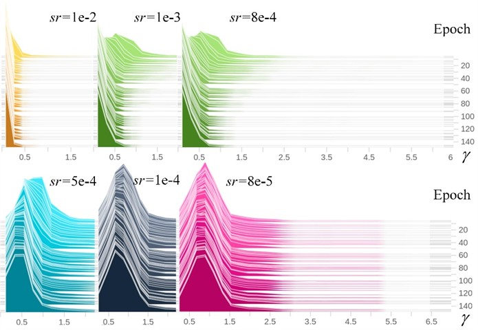
Fig. 7mAP at multi-degree sparsity rates
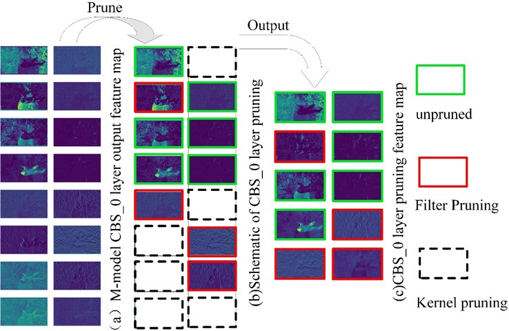
After determining the sparsity rate, this study performed pruning on the YOLOv5n model at different ratios to select the optimal pruning rate. Table 1 presents the changes in model parameters after pruning and fine-tuning at a sparsity rate of 8e-4 with various pruning rates. From the table, it can be observed that the number of model parameters, floating point operations, mAP, inference time with a batch size of 32, and model weight are all approximately negatively correlated with the pruning rate. However, in terms of inference time, there is a noticeable reduction when the pruning rate is 0.5, while the loss in mAP accuracy at this point is minimal. Therefore, a pruning rate of 0.5 is selected, which effectively compresses model parameters, reduces computational load, and significantly increases detection speed. At a pruning rate of 0.5, the output feature maps of each module in the YOLOv5n model changed in quantity before and after pruning, with the original output feature map counts being 16, 64, 128, and 256, corresponding to the pruned model's feature map counts of 10, 41, 83, and 167, respectively.
Table 1Model performance at different pruning rates
Pruning rate | Params(M) | FLOPs (G) | mAP (%) | FPS(b32) | Model weight (MB) |
0 | 1.767 | 4.176 | 98.2 | 1.82 | 3.8 |
0.1 | 1.604 | 3.779 | 98.3 | 1.77 | 3.5 |
0.2 | 1.420 | 3.340 | 98.0 | 1.82 | 3.1 |
0.3 | 1.232 | 2.914 | 97.6 | 1.67 | 2.7 |
0.4 | 1.056 | 2.514 | 97.5 | 1.49 | 2.4 |
0.5 | 0.878 | 2.129 | 97.2 | 1.28 | 2.0 |
0.6 | 0.708 | 1.748 | 96.3 | 1.36 | 1.7 |
0.7 | 0.532 | 1.312 | 94.0 | 1.23 | 1.3 |
0.8 | 0.353 | 0.917 | 91.7 | 0.97 | 1.0 |
0.9 | 0.177 | 0.502 | 86.7 | 0.77 | 0.6 |
To more intuitively observe the changes in output features after model pruning, the feature maps of the CBS_0 layer were visualized for comparison. The CBS_0 layer was selected because it has fewer channels and higher feature recognition, making it easier for the human eye to compare directly. As shown in Fig. 8. The original CBS_0 convolution layer mapped to 16 output feature maps, but after pruning, the number of output feature maps was reduced to 10. Based on the correspondence between the feature map outputs before and after pruning, the dashed boxes indicate the feature maps that disappeared corresponding to the filters being trimmed, the red boxes indicate that some convolution kernels in the filters were pruned, causing pixel changes in the corresponding feature maps, and the green boxes indicate the feature maps that remained consistent with the original model after pruning. After pruning, similar pattern feature maps were effectively trimmed. Applying pruning to the entire model significantly reduced the redundant parameters, greatly improving the model’s detection speed.
Fig. 8Output of feature map after pruning in CBS_0 layer
3.2. Model reconstruction results and analysis
This experiment compares several popular lightweight convolution modules, including DepthConv, GhostConv, GSConv, and the PConv used in this model. The CBS(Conv2d-BatchNorm-SiLU) module is the basic convolution module in YOLOv5, serving as a benchmark for the experiment. The experiment input values are generated by randomly sampling from a standard normal distribution to create a batch size of 8 and pixel matrices of size (512, 512), with both input and output channels set to 128 and a uniform convolution kernel size of 3×3. To reflect the modules’ actual performance, the warmup value is set to 500 and the number of tests is 1000. The module performance comparison is shown in Table 2.
Table 2Performance comparison of different lightweight convolution
Convolution module | Total time (s) ↓ | FPS ↑ | FLOPs (G) ↓ | Params (K) ↓ |
CBS | 14.83 | 13.48 | 310.31 | 147.84 |
DepthConv [21] | 31.75 | 6.30 | 38.92 | 18.30 |
GhostConv [22] | 16.55 | 12.09 | 19.46 | 9.15 |
GSConv [23] | 40.93 | 4.89 | 159.05 | 75.71 |
PConv [24] | 7.13 | 28.07 | 20.40 | 9.47 |
According to Table 2, PConv demonstrates the best inference speed and shows significant advantages in reducing both floating point operations and parameter count. Therefore, using PConv to reconstruct the C3 residual branch is a feasible approach. In the fusion experiments, the CPB module performed exceptionally well, with a noticeable reduction in parameter count compared to the C3 module. Table 3 illustrates the parameter count comparison between the C3 and CPB modules at layer X. In this experiment, we replaced the larger parameter modules C3_6, C3_8, and C3_23 in the original model with CPB_6, CPB_8, and CPB_23, resulting in model M, which achieved an accuracy of 98.2. This approach successfully minimized the model's parameter count while maintaining its accuracy.
Table 3Comparison of parameter counts at layer X
Modules | Backbone network module | Neck network module | ||||||
C3_X module | C3_2 | C3_4 | C3_6 | C3_8 | C3_13 | C3_17 | C3_20 | C3_23 |
Parameter | 4800 | 29184 | 156928 | 296448 | 90880 | 22912 | 74496 | 296448 |
Parameter reduction | ↓1392 | ↓11136 | ↓66816 | ↓89088 | ↓22272 | ↓5568 | ↓22272 | ↓89088 |
CPB_X module | CPB_2 | CPB_4 | CPB_6 | CPB_8 | CPB_13 | CPB_17 | CPB_20 | CPB_23 |
Parameter | 3408 | 18048 | 90112 | 207360 | 68608 | 17344 | 52224 | 207360 |
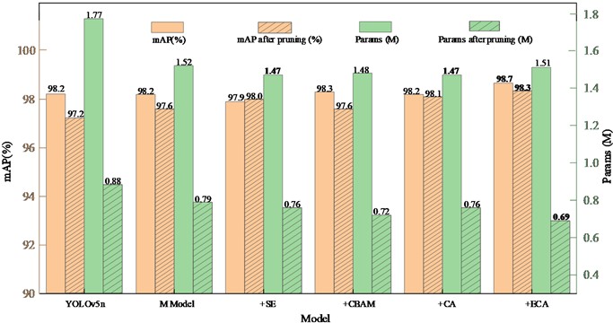
The CPB module aims to further reduce the parameters of the pruned model while keeping the changes in pruning accuracy minimal. This experiment employs a method of integrating attention modules to enhance the model’s detection accuracy by incorporating attention mechanisms into the C3_2, C3_4, and C3_20 layers of the baseline model M. To visually demonstrate the impact of different attention modules on the training accuracy before and after pruning, while offsetting the changes in network layers caused by the addition of attention mechanisms, this study compares popular attention modules such as SE [25], CBAM [26], CA [27], and the ECA attention module used in this research. As shown in Fig. 9.
The M model, obtained by integrating the CPB module with YOLOv5n, shows a significant reduction in the number of parameters both before and after pruning, while maintaining stable accuracy. By incorporating different attention mechanisms into the M model, the resulting pruned model demonstrates improvements in both accuracy and parameter count. Notably, the ECA attention mechanism stands out in this experiment, achieving a pre-pruning accuracy of 0.987 and a post-pruning accuracy of 0.983, with a significant reduction in parameter count to just 0.69M.
3.3. Final model performance analysis
To validate the performance of the final model in object detection, we lightweighted the model and evaluated it using mAP, parameter count, floating point operations, and FPS, with the results presented in Table 4. We employed the Sparse Group Lasso Prune method to achieve model sparsity and obtain the optimal sparse pruning parameters. Next, we replaced the CPB module using a pre-pruning method, ensuring that the pruned model’s weight was further reduced while maintaining stable accuracy. Finally, we integrated the ECA attention module, which improved the accuracy of the pruned model while also compressing the parameter count, resulting in the final model PCB-YOLOv5n-Prune. We also tested the detection performance of the model before and after pruning.
Fig. 9Performance comparison before and after pruning the reconstructed model
According to the data in Table 4, the YOLOv5n model after pruning has seen a reduction of approximately 50 % in both parameter count and floating point operations. At a batch size of 32, the model’s speed increased by about 246 FPS, but the mAP decreased by 1 %. By employing a pre-pruning method to replace the CPB module, the model’s accuracy further improved after pruning, while floating point operations and parameter count were reduced even more, with the speed increasing by an additional 54 FPS on top of the pruning improvement. After integrating the ECA attention mechanism, the inference speed decreased slightly due to the addition of 30 layers compared to model M, but it still showed a significant improvement over the original YOLOv5n, with accuracy similar to YOLOv5n. Furthermore, when combined with ByteTrack, the improved model’s detection frame rate increased by 39 FPS compared to YOLOv5n.
Table 4Ablation experiment
Model | CPB | prune | ECA | mAP (%) | Params(M) | FLOPs (G) | FPS(b32) | ByteTrack (FPS) |
Yolov5n | – | – | – | 98.2 | 1.76 | 4.1 | 534.7 | 57 |
prune | √ | – | – | 97.2 | 0.88 | 2.1 | 781.2 | 88 |
CPB | √ | √ | – | 97.6 | 0.79 | 1.9 | 836.0 | 92 |
ECA | √ | √ | √ | 98.3 | 0.69 | 1.8 | 785.0 | 96 |
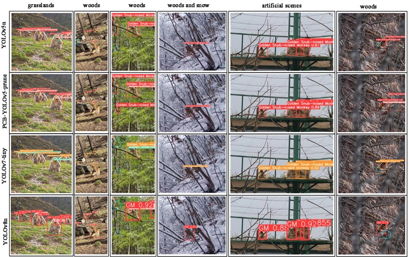
To validate the effectiveness of the model improvements, we selected images of golden snub-nosed monkeys taken in various backgrounds, including grasslands, forests, snowy scenes, and artificial settings, while considering occlusions. We compared the performance of the YOLOv5n, YOLOv7-tiny, YOLOv8n, and PCB-YOLOv5n-Prune models. Fig. 10 illustrates the detection results of golden snub-nosed monkeys in different real-world scenarios. From the figure, it is evident that the YOLOv5n, YOLOv7-tiny, and YOLOv8n models exhibited missed detections under various backgrounds, whereas the PCB-YOLOv5n-Prune model had significantly fewer missed detections. This model effectively improved detection rates in occluded situations by integrating an attention mechanism and also demonstrated a higher detection speed.
Fig. 10Scene occlusion detection comparison chart
To validate the performance of the algorithm presented in this paper within the public domain of object detection, we conducted experiments using the proposed network model on the PASCAL VOC dataset. The PASCAL VOC dataset is a significant benchmark in the field of computer vision, encompassing 20 common object categories such as people, animals, and vehicles. We adopted a popular training methodology by combining the training and validation sets from PASCAL VOC_2007 and PASCAL VOC_2012, resulting in a total of 16,551 images. The test set utilized the PASCAL VOC_2007 test set, which contains 4,952 images. Table 5 presents the test results of our algorithm alongside several mainstream networks on the PASCAL VOC dataset. All comparative experiments were conducted under identical environmental configurations. From Table 5, it is evident that our algorithm demonstrates competitive results in terms of model size and computational load compared to current networks. For instance, as shown in Table 5, our algorithm significantly improves detection accuracy compared to models based on the lighter ShuffleNetV2 backbone while maintaining a similar number of parameters and computational requirements. However, there remains a noticeable gap in detection accuracy when compared to larger models such as YOLOv7 and YOLOv5m. Additionally, when compared to transformer-based backbone models like EfficientViT and Swin Transformer, the detection accuracy is closely linked to their higher computational costs and longer training times.
Table 5Comparison experiments on the PASCAL VOC dataset
Models | Input | Parameters | FLOPs | mAP@0.5% | mAP@0.5:0.95% |
YOLOv7 | 640×640 | 37.2M | 105.4G | 81.5 | 63.1 |
YOLOv5m | 640×640 | 20.9M | 48.1G | 81.6 | 57.9 |
ShuffleNetV2 [28] | 640×640 | 1.02M | 0.6G | 47.5 | 25.9 |
EfficientViT [29] | 640×640 | 5.6M | 9.8G | 68.8 | 42.6 |
Swin Transformer [30] | 640×640 | 29.0M | 75.6G | 76.2 | 48.8 |
PCB-YOLO-prune | 640×640 | 0.71M | 1.8G | 69.1 | 41.7 |
The model primarily focuses on training for the characteristics of the golden snub-nosed monkey. To validate the improvements of the pruned network compared to other networks, we conducted comparative experiments using the golden snub-nosed monkey dataset with Faster R-CNN, YOLOv7-tiny, YOLOv8n, and YOLOv9c. The test results are shown in Table 6. We performed 150 tests on a single image sized 640×640 with a batch size of 1, and conducted another 150 tests at the same image size but with a batch size of 32. Additionally, we tested detection speed on a video lasting 5 seconds, which contained 150 frames, each sized 384×640, totaling 2.67 MB. The results indicate that our model outperforms other models in detection speed across various object specifications and demonstrates superior performance in video detection, making it particularly suitable for rapid detection of moving targets while maintaining accuracy that meets practical requirements.
Furthermore, we compared our model with other lightweight backbone models such as GhostNet and MobileNetV3 on the golden snub-nosed monkey dataset. Our model exhibited strong performance in terms of model weight, detection accuracy, and speed. Both GhostNet and MobileNetV3 utilize depthwise separable convolutions, which decompose standard convolutions into two steps: first convolving each input channel independently and then performing pointwise convolution (1x1 convolution). This design significantly reduces computational load and parameter count. However, the reduced number of parameters may lead to a decrease in the model's expressive power, potentially impacting accuracy.
In our model, the introduced CPB module incorporates partial convolution (PConv), which excels at preserving spatial information. It effectively reduces overall parameter count and computational load while maintaining model accuracy. The use of pruning further minimizes the model's cost. Additionally, the ECA module in our model replaces fully connected layers with one-dimensional convolutions, significantly lowering computational complexity and adaptively adjusting kernel sizes based on input features to better capture inter-channel dependencies. This design further enhances the detection performance of the model.
Table 6Performance of different algorithmic models
Model | mAP (%) | Params (M) | FLOPs (G) | FPS (b1) | FPS (b32) | FPS (2.67MB) | Model weight (MB) |
Faster rcnn | 92.0 | 28.3 | 474.1 | 27.3 | – | 76.3 | 113.4 |
YOLOv7-tiny [31] | 98.3 | 6.0 | 13.2 | 96.2 | 526.3 | 83.3 | 12.3 |
YOLOv8n | 98.4 | 3.0 | 8.1 | 58.5 | 158.6 | 90.1 | 6.3 |
YOLOv9c [32] | 98.8 | 50.7 | 236.6 | 23.8 | 52.7 | 29.6 | 102.8 |
Ghostnet | 97.2 | 1.3 | 2.9 | 126.9 | 447.9 | 128.2 | 2.9 |
MobileNetV3 [33] | 93.6 | 0.8 | 1.3 | 100.3 | 441.2 | 103.1 | 1.9 |
Ours | 98.3 | 0.7 | 1.8 | 120.8 | 785.0 | 129.9 | 1.7 |
3.4. Design of the visualization interface combined with ByteTrack
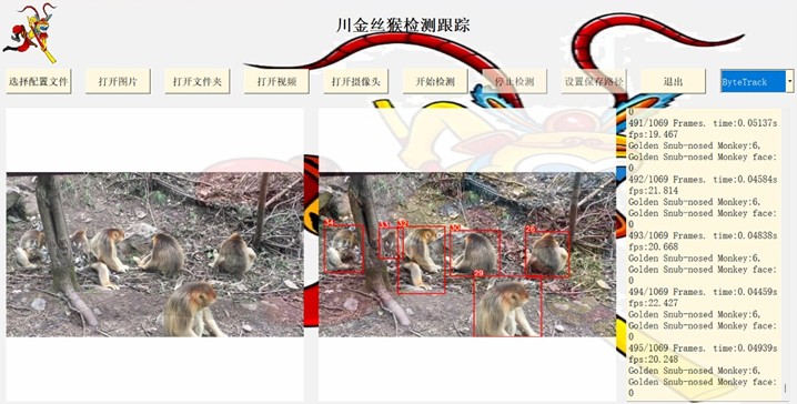
In this experiment, we utilized PyQt5 to encapsulate and package the proposed model. We converted the generated best.pt file into best.torchscript format using the official YOLOv5 export.py script, providing the necessary weight files for model visualization. The visualization interface includes options for selecting configuration files, opening different file formats, starting and stopping detection, setting the save path, and enabling tracking. The right side of the interface features settings for video frame segmentation, display of detection frame rates, target types, and the number of targets. The detection effect of deploying this model on low-performance devices is shown in Fig. 11.
4. Conclusions
This study focuses on the facial and body features of the golden snub-nosed monkey, integrating the YOLOv5n model with a pruning algorithm based on Sparse Group Lasso. By employing the CPB module, which utilizes Pconv and residual structures, we reconstructed the model to achieve rapid detection of individual golden snub-nosed monkeys. Additionally, the incorporation of the ECA attention mechanism improved detection performance for occluded targets, resulting in a pruned model accuracy of 0.983. Compared to the original model, the improved version reduced the parameter count by 1.07M, decreased computational load by 2.3G, and lightened the model by 2.3 MB, significantly enhancing detection speed. Moreover, we integrated ByteTrack with this lightweight model to enable continuous multi-target tracking of golden snub-nosed monkeys, enhancing the continuity of object detection.
Fig. 11Visualization interface for detection and tracking of golden snub-nosed monkeys
The improved YOLOv5n model has broad application potential in animal behavior observation, wildlife monitoring, and conservation efforts. It can be integrated into mobile devices for real-time capture and identification of animals, providing valuable data for ecological research. Deploying fixed monitoring systems in specific reserves allows for around-the-clock automated surveillance to promptly detect habitat destruction and illegal poaching activities. Furthermore, integrating this model into drone systems enables efficient monitoring over vast areas, particularly in hard-to-reach locations. The enhanced YOLOv5n model offers technical support for wildlife conservation by lowering hardware performance requirements and providing a reference for developing portable mobile terminals for golden snub-nosed monkey detection. This advancement can help researchers dedicated to golden snub-nosed monkey protection and study reduce labor costs and promote smart forestry development. Future work could combine visible light and thermal infrared sensors to further expand the dataset across different backgrounds, improving detection capabilities in complex environments.
References
-
M. Li and Z. F. Xiang, “Flagship species under China’s protection:golden monkeys,” (in Chinese), World Environment, No. S1, No. S1, pp. 12–15, May 2016, https://doi.org/cnki:sun:sjhj.0.2016-s1-005
-
X. J. Wang et al., “Species Associations and Conservation of Sichuan Snub-Nosed Monkey in the Tangjiahe National Nature Reserve,” (in Chinese), Chinese Journal of Wildlife, Vol. 44, No. 1, pp. 1–13, Aug. 2023, https://doi.org/10.12375/ysdwxb.20230101
-
H. Yao et al., “Endozoochorous seed dispersal by golden snub‐nosed monkeys in a temperate forest,” (in Chinese), Integrative Zoology, Vol. 16, No. 1, pp. 120–127, Oct. 2020, https://doi.org/10.1111/1749-4877.12488
-
X. Y. Wang and L. S. Zan, “Golden snub-nosed monkey biological characteristics, population, protection and research progress,” (in Chinese), Shaanxi Forest Science and Technology, Vol. 50, No. 1, pp. 102–107, 2022, https://doi.org/10.12340/sxlykj2022010021
-
M. Hussain, “YOLOv1 to v8: unveiling each variant-a comprehensive review of YOLO,” IEEE Access, Vol. 12, pp. 42816–42833, Jan. 2024, https://doi.org/10.1109/access.2024.3378568
-
Y. W. Xu, J. Li, Y. F. Dong, and X. L. Zhang, “Survey of the Development of YOLO Object Detection Algorithms,” (in Chinese), Frontiers of Computer Science and Technology, Vol. 18, No. 9, pp. 2221–2238, Jun. 2024, https://doi.org/10.3778/j.issn.1673-9418.2402044
-
N. Fang, “Research and implement of gold monkey recognition based on convolutional neural network,” (in Chinese), M.S. thesis, School of Computer Science and Technology, Xidian University, Xian, China, 2017.
-
G. W. Wang, “The research on face recognition of sichuan golden monkey,” (in Chinese), M.S. thesis, School of Electronics and Communication Engineering, Northwest University, Xian, China, 2018.
-
X. Hu, “Research and implementation of facial recognition of golden monkey based on attention mechanism,” (in Chinese), M.S. thesis, School of Computer Science and Technology, Xidain University, Xian, China, 2019.
-
R. Sun et al., “Optimized detection method for snub-nosed monkeys based on faster R-CNN,” (in Chinese), Laser and Optoelectronics Progress, Vol. 57, No. 12, pp. 259–268, 2020.
-
S. Ren, K. He, R. Girshick, and J. Sun, “Faster R-CNN: towards real-time object detection with region proposal networks,” IEEE Transactions on Pattern Analysis and Machine Intelligence, Vol. 39, No. 6, pp. 1137–1149, Jun. 2017, https://doi.org/10.1109/tpami.2016.2577031
-
Z.-Q. Zhao, P. Zheng, S.-T. Xu, and X. Wu, “Object detection with deep learning: a review,” IEEE Transactions on Neural Networks and Learning Systems, Vol. 30, No. 11, pp. 3212–3232, Nov. 2019, https://doi.org/10.1109/tnnls.2018.2876865
-
M. P. Mathew and T. Y. Mahesh, “Leaf-based disease detection in bell pepper plant using YOLO v5,” Signal, Image and Video Processing, Vol. 16, No. 3, pp. 841–847, Sep. 2021, https://doi.org/10.1007/s11760-021-02024-y
-
S. Puliti and R. Astrup, “Automatic detection of snow breakage at single tree level using YOLOv5 applied to UAV imagery,” International Journal of Applied Earth Observation and Geoinformation, Vol. 112, p. 102946, Aug. 2022, https://doi.org/10.1016/j.jag.2022.102946
-
F. Zhang, P. C. Zhang, L. Wang, R. H. Cao, and X. P. Wang, “Research on lightweight crested ibis detection algorithm based on YOLOv5s,” (in Chinese), Xi’an Jiaotong Univ, Vol. 57, No. 1, pp. 110–121, 2023, https://doi.org/10.7652/xjtuxb202301011
-
H. Sun, B. Wang, and J. Xue, “YOLO-P: An efficient method for pear fast detection in complex orchard picking environment,” Frontiers in Plant Science, Vol. 13, p. 10894, Jan. 2023, https://doi.org/10.3389/fpls.2022.1089454
-
W. H. Yang et al., “CCNN-swin transformer detection algorithm of forest wildlife images based on improved YOLOv5s,” (in Chinese), Journal of Computer Applications, Vol. 60, No. 3, pp. 121–130, 2024, https://doi.org/10.11707/j.1001-7488.lykx20220597
-
N. Simon, J. Friedman, T. Hastie, and R. Tibshirani, “A sparse-group Lasso,” Journal of Computational and Graphical Statistics, Vol. 22, No. 2, pp. 231–245, Apr. 2013, https://doi.org/10.1080/10618600.2012.681250
-
Q. Wang, B. Wu, P. Zhu, P. Li, W. Zuo, and Q. Hu, “ECA-Net: efficient channel attention for deep convolutional neural networks,” in IEEE/CVF Conference on Computer Vision and Pattern Recognition (CVPR), pp. 11531–11539, Jun. 2020, https://doi.org/10.1109/cvpr42600.2020.01155
-
Y. Zhang et al., “ByteTrack: multi-object tracking by associating every detection box,” in Lecture Notes in Computer Science, Cham: Springer Nature Switzerland, 2022, pp. 1–21, https://doi.org/10.1007/978-3-031-20047-2_1
-
M. Tan and Q. V. Le, “EfficientNet: rethinking model scaling for convolutional neural networks,” arXiv, pp. 6105–6114, Jan. 2019, https://doi.org/10.48550/arxiv.1905.11946
-
K. Han, Y. Wang, Q. Tian, J. Guo, C. Xu, and C. Xu, “GhostNet: more features from cheap operations,” in IEEE/CVF Conference on Computer Vision and Pattern Recognition (CVPR), pp. 1580–1589, Jun. 2020, https://doi.org/10.1109/cvpr42600.2020.00165
-
H. Li, J. Li, H. Wei, Z. Liu, Z. Zhan, and Q. Ren, “Slim-neck by GSConv: a lightweight-design for real-time detector architectures,” arXiv, Jan. 2022, https://doi.org/10.48550/arxiv.2206.02424
-
J. Chen et al., “Run, don’t walk: chasing higher FLOPS for faster neural networks,” in IEEE/CVF Conference on Computer Vision and Pattern Recognition (CVPR), pp. 12021–12031, Jun. 2023, https://doi.org/10.1109/cvpr52729.2023.01157
-
J. Hu, L. Shen, and G. Sun, “Squeeze-and-excitation networks,” in IEEE/CVF Conference on Computer Vision and Pattern Recognition (CVPR), pp. 7132–7141, Jun. 2018, https://doi.org/10.1109/cvpr.2018.00745
-
S. Woo, J. Park, J.-Y. Lee, and I. S. Kweon, “Cbam: Convolutional block attention module,” in Lecture Notes in Computer Science, Cham: Springer International Publishing, 2018, pp. 3–19, https://doi.org/10.1007/978-3-030-01234-2_1
-
Q. Hou, D. Zhou, and J. Feng, “Coordinate attention for efficient mobile network design,” in IEEE/CVF Conference on Computer Vision and Pattern Recognition (CVPR), pp. 13713–13722, Jun. 2021, https://doi.org/10.1109/cvpr46437.2021.01350
-
N. Ma, X. Zhang, H.-T. Zheng, and J. Sun, “ShuffleNet V2: practical guidelines for efficient CNN architecture design,” in Lecture Notes in Computer Science, Cham: Springer International Publishing, 2018, pp. 122–138, https://doi.org/10.1007/978-3-030-01264-9_8
-
X. Liu, H. Peng, N. Zheng, Y. Yang, H. Hu, and Y. Yuan, “EfficientViT: memory efficient vision transformer with cascaded group attention,” in IEEE/CVF Conference on Computer Vision and Pattern Recognition (CVPR), pp. 14420–14430, Jun. 2023, https://doi.org/10.1109/cvpr52729.2023.01386
-
Z. Liu et al., “Swin transformer: hierarchical vision transformer using shifted windows,” in IEEE/CVF International Conference on Computer Vision (ICCV), pp. 9992–10002, Oct. 2021, https://doi.org/10.1109/iccv48922.2021.00986
-
C.-Y. Wang, A. Bochkovskiy, and H.-Y. M. Liao, “YOLOv7: trainable bag-of-freebies sets new state-of-the-art for real-time object detectors,” in IEEE/CVF Conference on Computer Vision and Pattern Recognition (CVPR), pp. 7464–7475, Jun. 2023, https://doi.org/10.1109/cvpr52729.2023.00721
-
C.-Y. Wang, I.-H. Yeh, and H.-Y. Mark Liao, “YOLOv9: learning what you want to learn using programmable gradient information,” in Lecture Notes in Computer Science, Cham: Springer Nature Switzerland, 2024, pp. 1–21, https://doi.org/10.1007/978-3-031-72751-1_1
-
A. Howard et al., “Searching for MobileNetV3,” in IEEE/CVF International Conference on Computer Vision (ICCV), pp. 1314–1324, Oct. 2019, https://doi.org/10.1109/iccv.2019.00140
About this article
The authors have not disclosed any funding.
The datasets generated during and/or analyzed during the current study are available from the corresponding author on reasonable request.
Hao-Ran Xu is primarily responsible for enhancing the algorithm, conducting experimental training of the model, planning the research content, writing the paper, and creating the illustrations. Lei Wang and Peng-Chao Zhang are mainly responsible for the research findings and revisions of the paper. Kui Xiao is responsible for organizing the experimental data. Xing He and Yan Zhou are in charge of capturing the dataset and preprocessing the images.
The authors declare that they have no conflict of interest.
