Abstract
The development of a bridge damage detection method relies on comprehensive dynamic responses pertaining to damage. The numerical model of a bridge can conveniently considers various damage scenarios and acquire pertinent data, while the entity of a bridge or its physical model proves challenging. Traditional methods for identifying bridge damage often struggle to effectively utilize data acquired from diverse domains, presenting a significant hurdle in addressing cross-domain issues. This study proposes a novel cross-domain damage identification method for suspension bridges using recurrence plots and convolutional neural networks. By employing parameter identification-based modal modification of numerical model, the gap between numerical model and physical models eliminated. Un-threshold multivariate recurrence plots are used for accurately characterizing dynamic responses and extracting deeper damage features. Due to the scarcity of experimental data, which limits the training of robust neural networks, a transfer learning tailored for convolutional neural networks is implemented. This strategy not only addresses the issue of small sample sizes but also significantly enhances the network's ability to identify structural damage across diverse bridge domains. The proposed damage identification method is validated using a combination of numerical simulations and physical experiments on a specific single-span suspension bridge. Results demonstrate that un-threshold multivariate recurrence plots reveal detailed internal structure and damage information. Furthermore, the utilization of improved convolutional neural networks effectively facilitates cross-domain structural damage identification, marking a significant advancement in the field of structural health monitoring.
Highlights
- The scaled physical model of a single-span suspension bridge is established.
- The dynamic responses of bridges are described by un-threshold multivariate recurrence plot.
- The convolutional neural network is used to train the damage samples.
- Transfer learning is used to realize cross-domain damage identification between the physical and numerical model.
1. Introduction
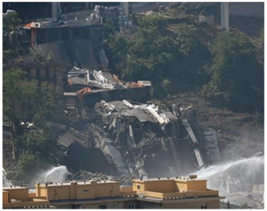
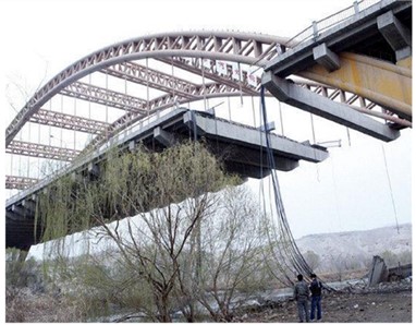
Bridges are a kind of important infrastructure related to people’s transportation and social development. The newly built bridges towards the direction of huge-number and large-scale with the rapid development of design and construction level [1]. However, in-service bridges inevitably suffer damage due to natural aging, disasters, and insufficient maintenance. Such damage significantly reduces the bridge’s load-bearing capacity, shortens its remaining lifespan, and even lead to catastrophic failures. For instance, as shown in Fig. 1(a), a 210-meter-long deck on Morandi Bridge collapsed when the steel cables could not withstand the force of gravity and snapped [2]. As shown in Fig. 1(b), the steel cables of the Kongquehe Bridge unintentionally connected the steel and aluminum to form a “galvanic corrosion battery”, which resulted in the breakage of the second boom of the main span and the destruction and collapse of the bridge deck [3]. Therefore, it is important to carry out in-time maintenance for operational bridges based on the detection of potential damage and monitoring of safety.
Fig. 1Examples of bridge accidents: a) Morandi Bridge in Genoa, Italy, b) Kongquehe Bridge in Korla, China
a)
b)
Many bridges are installed with structural health monitoring systems to obtain vibration data during daily operation. The information related to bridge damage are contained in these vibration data [4]. Some damage detection methods and damage indicators are established by analyzing the effects of different types and degrees of damage on structural vibration data [5]. Commonly, there are modal parameter-based methods represented by instantaneous frequency [6], damage detection methods based on model updating and parameter inversion [7, 8], damage detection methods based on dynamic fingerprint [9], and other damage indicators suitable for specific types of damage [10, 11]. These methods have generally been validated in laboratory-scale experiments [12] but have not yet been used in practical engineering. As the practically measured data is affected by environmental conditions, random loads, and external factors, the established detection methods cannot take these factors into account comprehensively and reasonably, resulting in the restricted promotion of these methods. The data collected by the bridge health monitoring system accumulates more and more over time. If the massive data is not timely and effectively converted into the information related to bridge safety, it becomes a burden to increase the operating cost. Recently, the rapid development of computing power and digital methods has brought new vitality to the analysis of bridge monitoring data. In particular, neural network technology represented by deep learning has gradually gained attention and has been widely used in the research of damage detecting such as concrete surface crack identification [13] and time series signal anomaly analysis [14]. Deep learning algorithms can extend common data to higher dimensions and explore the relationship between data features and bridge damage features in a high-dimensional space. Converting 1-D vibrational time series of bridges into 2-D images is a reliable way to improve the data dimension. This transform provides higher accuracy, higher noise immunity, and more efficient results for bridge SHM in terms of span damage identification.
The recursive nature, discovered by Poincaré in 1890 in the motion of celestial bodies [15], is a fundamental characteristic of many dynamic systems. Subsequently, Eckmann et al. [16] introduced the recurrence plots (RPs) to visualize the recursive nature exhibited by dynamic systems in high-dimensional phase space. To interpret the image features of the RPs and gain a deeper understanding of the characteristics embedded in signals, Zbilut and Webber [17] applied the recurrence quantification analysis to analyze features such as point density, distribution, and distances between points in recurrence plots. Then various extended types of recurrence plots are proposed, such as the un-threshold RPs [18], multivariate RPs [19], cross RPs, and joint RPs [20]. The vibrations of bridges also exhibit periodicity and recurrence subjected to external excitations such as pedestrian and vehicular loads. Nichols et al. [21] first performed the recurrence quantification analysis on vibration signals of thin plates forced by non-stationary excitations to extract damage features. Marwan et al. [22] demonstrated that RP contains relevant information about a dynamic system and verified that RP is a sensitive tool in complex systems. Samborski et al. [23] proposed a damage identification method based on frequency analysis and RPs, which is numerically verified based on cantilever, simply supported, and doubly clamped beams. Nevertheless, due to the difficulty of getting the sample sets of all kinds of damage in bridges, it is rarely to analyze and detect the bridge damages according to the RPs.
Deep neural networks, exemplified by Convolutional Neural Networks (CNNs), exhibit superior capabilities in information extraction, feature classification, and adaptive learning [24]. The CNNs are particularly adept at extracting latent intrinsic features from complex dynamic response data, yielding end-to-end automated identification of structural damage. Consequently, research on structural damage identification supported by CNNs attracts a lot of attention attentions. Lee et al. [25] developed a CNN-based damage localization method based on a numerical model of the Rahmen Bridge with the achievement of an 87.3 % identification accuracy. Zhan et al. [26] investigated the impact of structural parameter randomness on the accuracy of CNN-based damage identification. Sony et al. [27] proposed a multilevel method using windowed 1D-CNNs to detect the damages of pier settlement and tendon breakage. Das and Guchhait [28] embedded a 2D-CNN architecture into a deep learning algorithm for detecting the damage of a steel frame. He et al. [29] combined CNNs with recurrence plots to form a damage identification method, of which the effectiveness is validated by a scaled model of a three-span continuous beam bridge. Although the effectiveness of the combination of recursive analysis and deep learning to extract and separate damage-sensitive features from dynamic responses is proved, there are still some challenges exist: (i) the actual bridge and the finite element model are independent of each other, resulting in different dynamic responses even under the same operating conditions; (ii) parameter selection, which brings different damage identification results when dealing with small damage, is involved in traditional recursive analysis; (iii) few damage samples and sparse damage information of actual bridge are available.
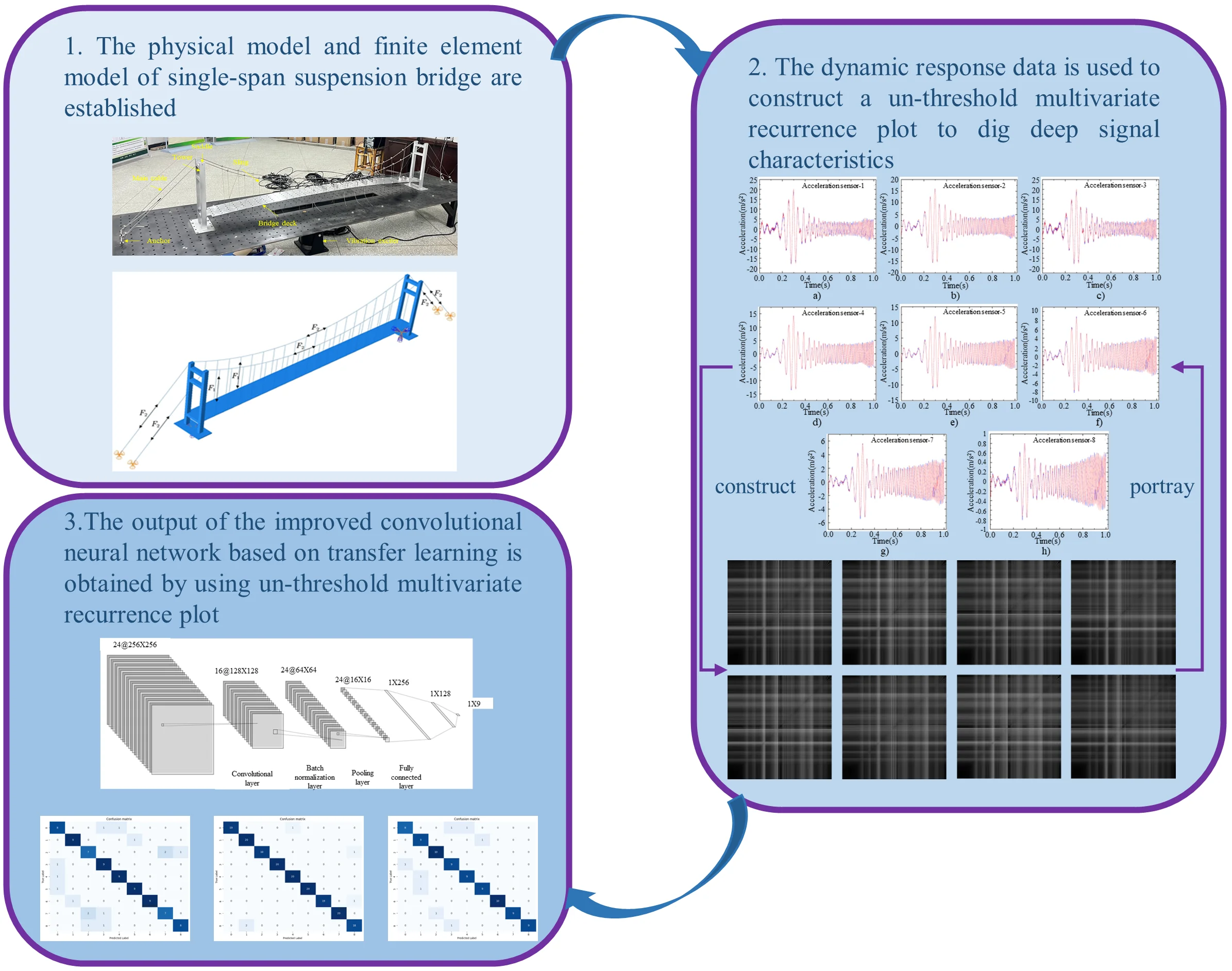
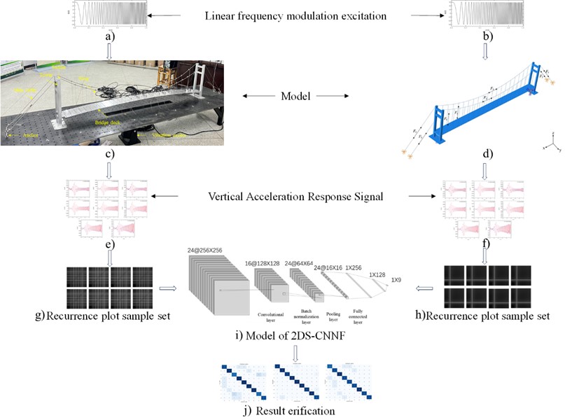
To address these issues, this study proposes a novel algorithm for bridge damage detection from the vibrational responses based on the recurrence plots and CNNs. First, the numerical model is updated with a Bayesian inference optimization algorithm, then the mutual transfer learning between the numerical model and the physical model is carried out, and finally the un-threshold recurrence plots are combined with CNNs to identify the bridge damage. A suspension bridge model is used to verify the feasibility and effectiveness of the proposed detection method. The rest of this paper is organized as follows: Section 2 formulates the proposed detection method; Section 3 introduces the numerical and physical suspension bridges and clarifies the damage setting; Section 4 constructs the sample spectra and CNN networks; Section 5 detects the damage in the physical suspension bridge using the established CNN networks; Section 6 summarizes the conclusions and further research.
2. Methodology
2.1. Fundamentals of recurrence plots
The recurrence plot (RP) is a visualization tool used to transform a time series data into a 2-D matrix that compares each point in a two-dimensional space to the others. Each point in the matrix represents the degree of similarity between two moments in time, typically depicted using binary or grayscale values. RP helps intuitively understand the repetitive patterns and dynamic features hides in the time series, making it extensively applicable in fields of signal processing, time series analysis, and dynamical system modeling.
For time series , the first step in constructing the RP is to reconstruct the equivalent phase space based on the time delay and embedding dimension . The time delay and embedding dimension can be determined through embedding dimension theory and time delay methods:
where, is the trajectory length of the reconstructed phase space, and is the number of time series
In phase space , the recurrence plot of time series x is constructed according to Eq. (2):
where, is the value at the position , is a predefined threshold distance, indicates the Euclidean distance between phase points in the reconstructed phase space. denotes the Heaviside function, which can be expressed below:
where, represents the distance calculated between points and in the reconstructed phase space. represents a black point at the position and represents a white point at the position .
The time delay can be determined by the mutual information method [30, 31]:
where, , are the single probability densities associated with the time series and , is the joint probability density associated with the time series and . The first local minimum of the mutual information curve is the optimal choice of .
The minimum embedding dimension can be determined by the false nearest neighbors [32]. With the time delay and the time series , an -dimensional state space vector is constructed. is denoted as the th neighbor of , the distance between them is defined as:
As the dimension of the embedding space increases from to , the distance between and can be expressed as:
The relative increment of the distance between and is calculated as:
where is the error threshold. When Eq. (8) is satisfied, points that were previously considered as neighbors now exhibit their true distances upon increasing the embedding dimension, suggesting that these points are not actually close in the higher-dimensional space. Such points are referred to as false nearest neighbors. The false neighboring point is easier to identify when 10 during the calculation process. When 1, it is called the nearest neighbor point. With the increase of the embedding dimension, when the number of false nearest neighbor points tends to 0, the embedding dimension currently is determined as the minimum embedding dimension .
To avoid the influence of the selection of thresholds and enhance the ability to handle multidimensional data, the traditional RP is modified.
The joint RP considers the recurrences of multiple variables’ trajectories within their respective phase spaces. The joint RP compares the similarity of recurrence natures among multiple dynamical systems. The joint RP of two signals is taken as an example, and are the reconstructed phase spaces, joint RP is described as:
The un-threshold RP calculates recurrences directly based on the similarity of time series data without presetting a threshold. The construction of the un-threshold RP is as follows:
where represents the distance between points and in the time series, which is typically calculated using the Euclidean distance.
In un-threshold RPs, each value directly affects the brightness or color of the corresponding pixel in the plot. Typically, smaller distances result in brighter pixels, indicating greater similarity between the states at two time points. The un-threshold RPs allow the intuitively repeating patterns and dynamic structures in time series data easily to be identified without the requirement of selecting an appropriate threshold.
2.2. Convolutional neural networks
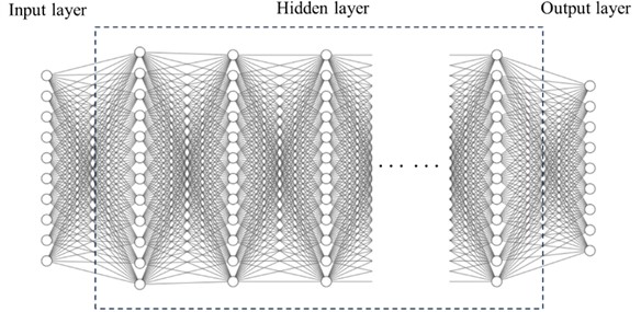
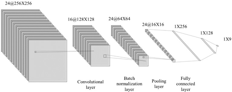
Convolutional Neural Networks (CNNs) are deep learning models inspired by the biological visual cortex. Aiming at simulating the human visual system for feature extraction, CNNs are primarily used for processing image data. As shown in Fig. 2, the deep learning network framework consists of an input layer, hidden layer and output layer. The hidden layer includes convolution layer, pooling layer and fully connected layer. The architecture of CNNs allows for parallel computing which can enhance computing efficiency.
CNNs are a type of multilayer feedforward neural network named for their use of convolution operations. CNNs extract and abstract image features effectively, making them suitable for tasks like image classification and object detection. Through convolution and pooling operations, CNNs achieve invariance to the positioning of targets within images. CNNs are widely applied and perform excellently in image processing and computer vision.
To ensure the network can capture the nonlinearities and complex dependencies in the input data, and to perform a variety of complex prediction and classification tasks, activation functions are set up in CNNs. The activation function used in this study is the Leaky ReLU, which addresses some issues associated with the standard ReLU function, such as failing to activate neurons from negative inputs and non-centered outputs. Leaky ReLU introduces a leaky value for negative values, ensuring that the count backward is never zero and thus resolving the problem of neurons failing to activate with negative inputs. The construction of the ReLU is as follows:
Non-linear activation functions add non-linearity to convolutional neural networks, enabling them to approximate virtually any function.
Fig. 2Architecture of deep learning network
2.3. Damage identification method
The differences between the numerical model of a suspension bridge and its physical model exist, despite the modal modifications to the numerical model. A CNN trained only on data from the numerical model may perform suboptimal when recognizing data obtained from physical model experiments, resulting in insufficient accuracy in cross-domain structural damage identification. To address this problem, this study proposes a cross-domain CNNs fusion (2D-CNNFs) method based on transfer learning [33] to release the single-domain data training and difficult cross-domain identification.
The domain in transfer learning, the subject space of knowledge learning, can be defined as:
where, and are the feature space and edge probability distribution, respectively.
The task of knowledge learning in transfer learning can be defined as:
where, and are the implicit characteristic function and label space, respectively. There are two types of agent space, active domain and target domain, and the probability distribution at the edge of agent space is different, which is expressed as .
The source task is a labeled source domain data , which can be represented as:
where, is the th data in the source domain feature space, is the th label in the source domain space, and is the number of samples in the source domain space.
The target task is an unlabeled target domain data , which can be expressed as:
Due to the similar features in the source domain and the target domain, transfer learning makes full use of the samples in the source domain to fit a decision function . Therefore, the can not only represent the mapping relationship between data and labels in the source domain, but also can be transferred to the target domain to express such mapping relationship and predict labels.
By comparing data across domains, common or similar features are found and thereby the transfer learning to enhance the network model can be applied. The trained network can generalize and apply the learned insights in different contexts to solve cross-domain structural damage identification problems [34, 35]. Based on the 2D-CNNs model and the idea of transfer learning, a cross-domain data feature cross transfer learning network model is constructed to achieve cross-domain structural damage identification. The flowchart of this method is illustrated in Fig. 3, and the detailed steps are drawn below.
Step 1: collecting accelerations of the physical model and the modified numerical model forced by frequency-swept excitations to obtain data set. The collected accelerations are extracted valid data points during the excitation period to form an 8-column by 1000-row numerical matrix.
Step 2: constructing the un-threshold multivariate RPs samples based on both the physical and numerical models.
Step 3: training the 2D-CNNs model using the numerical model-based RPs samples until the loss function stabilizes while the trained 2D-CNNs model is validated using 1/9 of the RPs samples.
Step 4: the set of physical model-based RPs samples is split into training and validation sets in a 1:1 ratio. The initial layers of the trained 2D-CNNs are frozen, and the end layers with the physical model-based samples are trained and validated to form the2D-CNNFs.
Step 5: inputting the un-threshold multivariate RPs from the physical model into the 2D-CNNFs for realizing the cross-domain structural damage identification.
Fig. 3Flowchart of damage identification method based on RPs and 2DS-CNNFs
3. Descriptions of a suspension bridge
3.1. Physical model
The load-bearing process of a suspension bridge is to transfer the external load from the deck to the slings and then to the main cables. The main cables, towers, and anchors constitute the primary load-bearing structure of a suspension bridge. The main cables distribute the shear forces to the bridge tower and transmit the axial forces to the foundation through the anchors connected to the ground. Other components of a suspension bridge include the stiffening girders of the bridge deck, slings, and saddles.
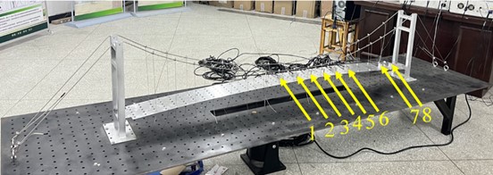
As shown in Fig. 3(c), the scaled model of a suspension bridge is prepared. The primary components selected for manufacturing the model include perforated aluminum plates, steel ropes, steel towers, clamps, and buckles. The main cables of the model are connected to the ground using buckles. The towers of the model and the work platform, as well as between the bridge deck and the main towers, are bolted together. The main cables are anchored at the top of the towers in notches to secure them. Clamps are used at the connections between the slings, main cables, and the bridge deck. The detailed dimensions of the physical model are listed in Table 1.
Table 1Geometrical dimensions of the suspension bridge model
Type | Values (mm) |
Bridge length | 3200 |
Main cable span | 2000 |
Main cable diameter | 4 |
Sling diameter | 2 |
Sling spacing | 10 |
Pylon height | 500 |
Bridge deck width | 100 |
Bridge deck thickness | 2 |
3.2. Numerical models
An equal-size finite element model of the suspension bridge was created using Abaqus software. This finite element model consists of four main components: the main cables, bridge towers, slings, and the bridge deck. Fixed constraints are set up at the bottom of the towers, between the bridge deck and the towers, between the tower and the main cable, and between the main cables and slings. Coupling interactions are established between the bridge deck and the slings. Translational displacement is fixed between the main cables and the foundation, while rotational directions are simulated with spring constraints with a spring stiffness of 1×10⁷N/m to mimic the physical model’s buckle. As the main cables and slings are the primary load-bearing components of the suspension bridge, they initially suffer tensile forces when subjected to constant loads. To accurately model the bridge’s operational state, axial prestress with 20 N and 1 N are assigned to main cables and slings, respectively. The material parameters of the numerical model are outlined in Table 2.
Table 2Material parameter of the numerical model
Bridge members | Density (tonne/mm3) | Elastic module (MPa) | |
Bridge deck | 2.70×10⁻⁹ | 50000 | 0.3 |
Tower | 7.85×10⁻⁹ | 206000 | 0.3 |
Main cable | 7.85×10⁻⁹ | 200000 | 0.3 |
Sling | 7.85×10⁻⁹ | 200000 | 0.3 |
During the discretization the finite element model, the bridge towers and deck are simulated using eight-node 3-D solid elements, specifically the C3D8R element in Abaqus software. The main cables and slings are simulated using truss elements T3D2, which is good at simulating the tensioned structural characteristics of components. The diameters of the main cables and the slings are set as 4 mm and 2 mm, respectively. The deck thickness is divided into four layers of mesh, and the mesh density is increased at various connection points and at the grooves at the top of the towers. The discretized model comprises a total of 5376 elements and 8591 nodes.
Fig. 4Numerical models of the suspension bridge: a) geometric model, b) discretized model
a)
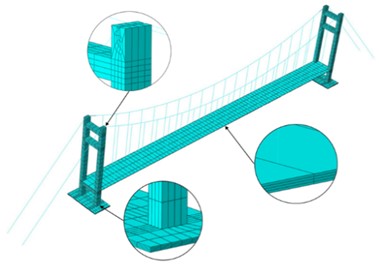
b)
3.3. Model modification
Seven frequencies of the physical model are identified from the frequency response functions derived by the modal testing data. The obtained seven frequencies are checked as the vertical bending and torsion modes of the model. For consistency, the modal order in the previous 50 orders of modal analysis of the numerical model is extracted and compared. The model modification based on parameter identification is employed to improve the fit between the finite element model and the physical model of the suspension bridge. A surrogate model is used to approximate the mechanical behavior of the numerical model while enhancing computational efficiency.
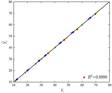
Among many optical algorithms, support vector regression (SVR) offers better handling of nonlinear relationships and noisy data, exhibiting significant generalization capabilities and largely avoiding data overfitting. Therefore, this study utilizes an SVR-driven Bayesian inference optimization algorithm for parameter identification to adjust the numerical model. The accuracy of the surrogate model is evaluated using the R-Squared (R2) error as follows:
where, is the actual observed value, is the value predicted by the model, is the mean of the actual observed value, and is the number of samples.
As shown in Fig. 5(a), the frequency curves constructed from the numerical natural frequencies has been revised. Moreover, the measured natural frequency data points fit better with the updated computational frequency curve after the model modifications. The parameter identification method effectively modifies the numerical model of the suspension bridge, making it more closely align with the actual physical model. As shown in Fig. 5(b), the 99.9 % validation accuracy of SVR proxy model demonstrates the numerical model of suspension bridge is well modified and can be used for cross-domain learning with the physical model.
3.4. Damage settings
Slings are critical load-bearing components of suspension bridges which suffer substantial loads. Slings are susceptible to aging and damage due to oxidation and corrosion from long-term exposure to natural elements. Moreover, significant wind loads, and bridge vibrations can cause instability to sling. Thus, slings are the most damage-prone components among the components of suspension bridges.
Fig. 5The results of model modification: a) measured frequency before and after modification, b) scatter plot of suspension bridge real response and surrogate model predicted response
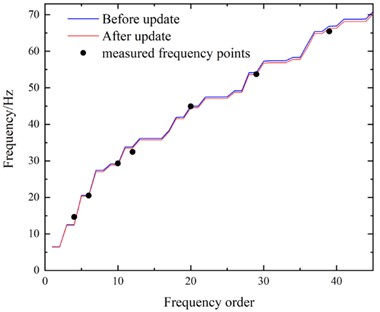
a)
b)
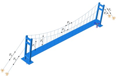
This study focuses on the damage of the slings in suspension bridges. Half of the bridge is investigated considering the symmetrical structure of the suspension bridge. As shown in Fig. 6(a), four distinct positions are considered with two severity levels, 9 cases are formed in total with the comparison of intact case. The damage locations are strategically set to cover a broad range of potential damage locations on the slings. Position nears the bridge tower, position locates at one-quarter of the bridge span from the tower, position locates at two-thirds of the span from the same side, and position locates at the midpoint of the span. When dealing with the physical model, damage is simulated by changing the slings to modify their elastic modulus. The severity of damage is simulated by using aluminum wire and nylon wire with different materials to replace the original steel wire. The damage using the aluminum wire and nylon wire are labeled as Type 1 and Type 2, respectively. As shown in Fig. 6(b), 8 accelerometers numbered from 1 to 8 are attached along the horizontal axis for measuring the vertical accelerations. The vertical accelerations of the corresponding nodes in the modified numerical model are extracted.
Fig. 6Damage settings: a) damage locations, b) accelerometers layout
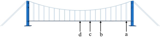
a)
b)
Table 3Damage scenarios
Case label | Damage location | Damage severity |
1 (intact case) | / | / |
2 | b | Type 1 |
3 | c | Type 1 |
4 | d | Type 1 |
5 | a | Type 1 |
6 | b | Type 2 |
7 | c | Type 2 |
8 | d | Type 2 |
9 | a | Type 2 |
4. Construction and verification of sample spectra
4.1. Data collection and processing
As shown in Fig. 7 (a), a linear frequency-swept excitation is applied on the bridge physical model using an electromagnetic shaker. The frequency of the excitation increments from 0 to 100 Hz in 10 seconds, while the sampling frequency of the signal acquisition is set to 1000 Hz. Each damage case is reloaded 20 times, totally 180 sets of vertical accelerations are collected. Fig. 7(b) shows one of the accelerations sets.
Fig. 7a) linear frequency-swept excitation, b) acceleration responses

a)
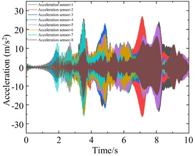
b)
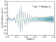
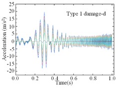
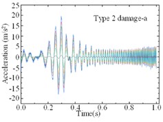
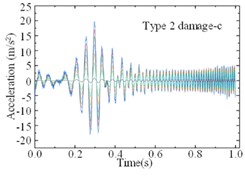
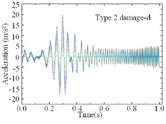
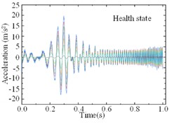
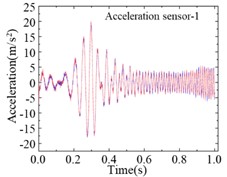
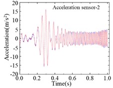
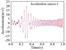
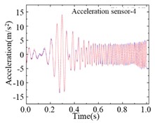
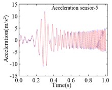
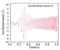
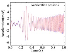
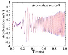
For the modified numerical model, a same linear frequency-swept excitation ranging from 0 to 100 Hz is also applied at the center of the bridge deck. The transient analysis is conducted on the modified numerical model, with a sampling frequency of 1000 Hz and a sampling duration of 10 seconds. Each of the 9 damage cases is subjected to 200 computational analyses, and a total of 1800 sets of vertical accelerations are collected. Fig. 8 displays the computational results for different damage cases under the same excitation. Various cases show similar vibration characteristics under the same excitation, it is difficult to find the differences directly from the time-domain accelerations. Fig. 9 shows the computational results of different sensors for the type 1 damage-a damage case under excitations-1 and excitations-2 The amplitudes of accelerations induced by different excitations show some difference, and the frequency variations remain highly consistent. Regarding the different damage cases and measuring positions, the variations of accelerations are weak, and it is not enough to deconstruct and observe this difference in 1-D signals.
Fig. 8Accelerations forced by a same excitation for different damage cases
a)

b)

c)
d)
e)

f)
g)
h)
i)
Fig. 9Accelerations of different measuring positions for same damage case
a)
b)
c)
d)
e)
f)
g)
h)
4.2. Sample spectra of un-threshold RPs
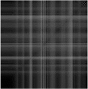
To minimize the loss of signal characteristics caused by parameter settings, the un-threshold multivariate RPs have been employed to extract structural damage characteristics. The un-threshold multivariate RPs allow a more nuanced representation of the damage by capturing a broader range of interactions between multiple variables without the requirement of predefined thresholds. An 8-dimensional un-threshold multivariate RPs using accelerations from each set of experiments are constructed according to Eq. (10) with the following steps.
Step 1: data preparation. Standardizing the data and transforming it into a standard normal distribution with the same mean and standard deviation as:
where, is the original data point, is the mean of the dataset, and is the standard deviation of the dataset. The resulting Z-value indicates the deviation of the original data point from the mean, expressed in units of standard deviation.
Step 2: RP construction. Calculating the number of RPs that can be generated based on the size of the input matrix, the dimensions of the RPs, and the step size.
Step 3: distance calculation. Creating a three-dimensional zero matrix to store the distances for each RP. Calculating the Euclidean distance between each block and storing these distances in the three-dimensional zero matrix.
Step 4: image conversion and saving. Converting each distance matrix within the three-dimensional zero matrix into a grayscale image, thereby constructing the un-threshold multivariate RPs.
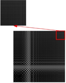
Fig. 10 shows the un-threshold multivariate RPs based on the modified numerical model of the suspension bridge, which depict the same locations with different severities of damage. The primary differences in damage depiction are concentrated in the upper right corner of the plots. In Fig. 10(b) and Fig. 10(c), there is a consistent “cross” feature at the positions indicated by the rectangle, although this feature exists in different spatial dimensions. This specific feature indicates the potential areas of structural damage and could be used to identify and quantify damage severity.
Fig. 10Un-threshold multivariate RPs for different cases based on the modified numerical model
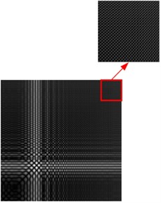
a) Health state
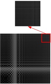
b) Type 1 damage-c
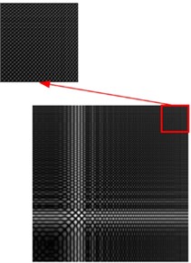
c) Type 2 damage-c
Fig. 11 shows un-threshold multivariate RPs based on the modified numerical model of the suspension bridge, which depict different locations with the same severity of damage. A “cross” feature is noticeable at the position indicated by the rectangle in the upper right corner of the RPs. However, variations in the image’s grayscale and spatial dimensions can be observed. These differences reflect the influence of the position of damage on the structural dynamics captured by the RPs. This suggests that the “cross” feature is a consistent marker of damage and it changes depending on the location of the damage within the structure.
Fig. 11Un-threshold multivariate RPs for the different locations based on the modified numerical model
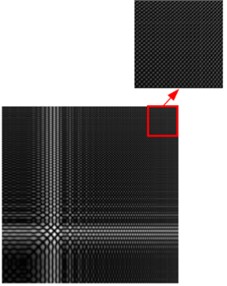
a) Type 2 damage-a
b) Type 2 damage-d
Fig. 12 shows the un-threshold multivariate RPs constructed from the measured data of different cases using the physical model. The differences in grayscale can be used to distinguish between the severities and specific characteristics of the damage. The visual diversity in the RPs highlights the utility of this method in capturing subtle nuances in bridge’s behavior, which can be critical for accurate damage detection.
Fig. 12Un-threshold multivariate RPs for different cases based on the physical model
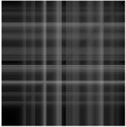
a) Health state
b) Damage state
In summary, the two-dimensional RPs release varying damage characteristics, which confirms the effectiveness for depicting structural damage in single-span suspension bridges. Fig. 11 and Fig. 12 illustrate some differences for different damage scenarios, but the distinctness of these features is not easily discernible to the naked eye. To address this issue, it is proposed to utilize the powerful classification capabilities of CNNs for image classification, aiming to enhance damage identification in structural assessments.
Table 4Numbering corresponding to operating conditions
Tag number | Operating conditions (2D-CNN) | Operating conditions (2D-CNNF) |
0 | Intact | Type 1, damage-c |
1 | Type 1, damage-c | Type 2, damage-c |
2 | Type 1, damage-b | Intact |
3 | Type 1, damage-d | Type 1, damage-b |
4 | Type 1, damage-a | Type 2, damage-b |
5 | Type 2, damage-c | Type 1, damage-d |
6 | Type 2, damage-b | Type 2, damage-d |
7 | Type 2, damage-d | Type 1, damage-a |
8 | Type 2, damage-a | Type 2, damage-a |
1800 un-threshold multivariate RPs based on the modified numerical model and 180 RPs based on the physical model are used to construct two pre-training sample sets.
The first set comprises only the RPs from the modified numerical model and is intended for a 2DS-CNN network model. The RPs are classified into 9 categories according to their scenarios, with each training set containing 180 plots and each validation set containing 20 plots, labeled from 0 to 8 as listed in Table 4. The second set, intended for a 2DS-CNNF network model, includes RPs from both the physical model and the modified numerical model. Similarly, the RPs are classified into 9 categories, each containing 190 training plots and 30 validation plots.
4.3. 2D-CNNFs structure and parameter settings
The structure of the CNN model adapted in this study, which incorporates the convolutional layer, batch normalization layer, pooling layer, and fully connected layer, is depicted in Fig. 13. The batch normalization layer helps standardize the inputs across the network, facilitating faster and more stable training. This configuration is aimed at optimizing the network's performance in recognizing and interpreting the complex patterns represented in the RPs. To prevent overfitting due to excessive complexity while ensuring robust feature extraction capabilities, three convolutional layers are chosen. The batch normalization layers, placed after the convolutional layers, address the issue of vanishing gradients during training, which can slow network convergence, thereby enhancing the robustness of the CNN. Additionally, the Leaky ReLU function is used as the activation function, enhancing the network's capability for nonlinear modeling.
Fig. 13Structure of the CNN modal
The CNNs are trained using un-threshold multivariate RPs generated from data collected with the modified numerical model of the suspension bridge as input and validation samples. The network’s parameters are detailed in Table 5. The setup allows comprehensive testing of the CNN’s effectiveness in detecting and classifying structural damage based on complex patterns identified in the RPs.
5. Damage identifications
5.1. Improvement of CNNs based on transfer learning
The data of various damages can be obtained easily from the numerical model, but not easily from the physical model or real bridge. To address the difficulty of obtaining extensive physical model damage data for input training, the transfer learning is utilized. Transfer learning approach allows a cross-domain data feature fusion for achieving an effective damage identification in the physical model. The transfer learning network model, abbreviated as CNNF, is established, and its framework is illustrated in Fig. 14. The changes to the model’s end-layer parameters are detailed in Table 6.
Table 5Parameter settings of the CNNs
Model parameter | Value | Parameter description |
dimension | 224×224 | Input image dimension |
in_channels | 1 | The number of channels for the input image, where a grayscale image is used |
out_channels (conv1) | 8 | The number of output channels of the first convolution layer |
kernel_size (conv1) | 11 | The size of the convolution kernel of the first convolution layer |
stride (conv1) | 2 | The step size of the first convolution layer |
out_channels (conv2) | 16 | The number of output channels of the second convolution layer |
kernel_size (conv2) | 5 | Convolution kernel size of the second convolution layer |
stride (conv2) | 2 | The step size of the second convolution layer |
out_channels (conv3) | 32 | The number of output channels of the third convolution layer |
kernel_size (conv3) | 5 | The convolution kernel size of the third convolution layer |
stride (conv3) | 2 | The step size of the third convolution layer |
in_features (fc1) | 32*36 | The number of input features for the first fully connected layer |
out_features (fc1) | 64 | The number of output features of the first fully connected layer |
out_features (fc2) | 9 | The output dimension of the second fully connected layer (Classification number) |
criterion | CrossEntropyLoss | Cross entropy loss function |
optimizer | Adam | Use the Adam optimizer |
learning rate | 0.001 | Learning rate of the optimizer |
num_epochs | 150 | The number of rounds when training the model |
train(batch_size) | 1620 | Batch size of the training data loader |
val(batch_size) | 180 | Verify the batch size of the data loader |
data_split | 9:1 (train:test) | The data set is divided into train and val in a 9:1 ratio |
Several key steps of the construction of the CNNF involves:
Step A: source domain training.
A total of 1800 labeled RPs from the numerical model of is used to train the 2D-CNNs, among them 1/9 of the data is split as validation sets. This step aims to extract structural damage features and establish mapping relationships. The trained model provides a pretrained network for the transfer of learning from numerical features to physical features.
Step B: fine-tuning with mixed data.
The parameters of the front layers of the 2D-CNNs are frozen to retain the damage features from the numerical model. A small number of labeled physical RPs are input into the network's end layers for rapid training. This process fuses the features from both the numerical model and physical model and realizes the preparation of the 2D-CNNFs.
Step C: unlabeled data testing.
This step involves inputting unlabeled physical RPs into the trained 2D-CNNFs to observe prediction outcomes and validate the new network model’s accuracy and robustness.
Using the framework of the 2D-CNNF network, a large number of the modified numerical data, along and a small number of physical data are used for training and validating. This approach is robust and effective for structural damage identification with limited actual damage data.
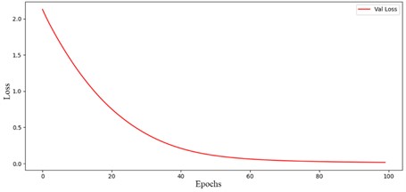
Based on the trained 2D-CNNs, 180 un-threshold multivariate RPs constructed from physical model of the suspension bridge are used. The training and validation data were split equally for training in the end layers of the constructed 2D-CNNs. 10 RPs are randomly selected from each case, and a validation set is formed by a total of 90 RPs. As shown in Fig. 15, the loss function of the improved convolutional neural network approaches zero, demonstrating that the network effectively extracted image features from the un-threshold multivariate RPs. It also successfully integrated the features of the modified finite element model, resulting in a cross-domain 2DS-CNNFs.
Fig. 14Framework of 2D-CNNFs
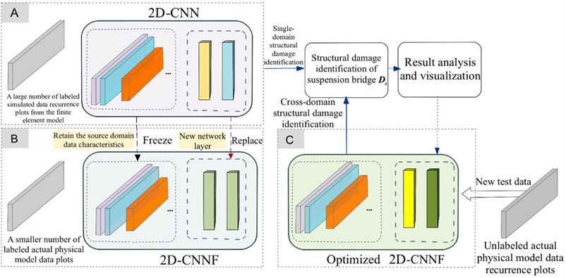
Table 6Parameter configuration of the terminal layer
Model parameter | Value | Parameter description |
num_epochs | 100 | The number of rounds when training the model |
train(batch_size) | 90 | Batch size of the training data loader |
val(batch_size) | 90 | Verify the batch size of the data loader |
data_split | 1:1 (train:test) | The data set is divided into train and val in a 1:1 ratio |
Fig. 15Function plot of loss: a) train loss, b) validation loss
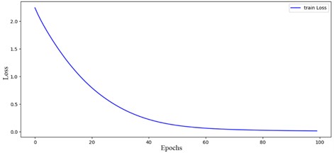
a)
b)
5.2. Identification results
The confusion matrix derived by the 2D-CNN based on the validation data is shown in Fig. 16. The main diagonal of the matrix shows an accuracy of 97.2 %, indicating that the trained 2D-CNN can effectively extract the features from the un-threshold multivariate RPs. The 2D-CNNFs generated the numerical data and physical data are compared with the 2D-CNNs generated by the numerical data. Both networks are used to identify damage using un-threshold multivariate RPs generated from physical data of the suspension bridge, with the results displayed in Fig. 16 and Fig. 17.
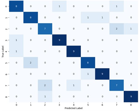
Fig. 17 reveals a damage identification accuracy of 83.3 %, indicating that the RPs generated from the modified numerical data indeed share similar features with those generated from physical data of the suspension bridge. However, the accuracy of the damage identification is defective during the cross-domain structural damage identification. Specifically, the identification accuracy of the intact case and type 1 case achieves only 77.8 %. The confusion between these two cases suggests that the 2D-CNNs without cross-domain feature learning struggles to distinguish between the two types of damage.
Fig. 16Confusion matrix for damage identification in modified finite element model
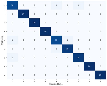
Fig. 17Confusion matrix for non-transfer learning group
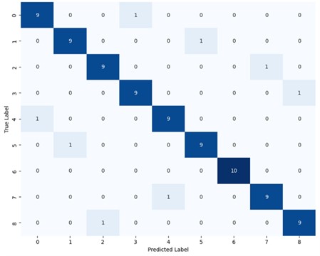
In contrast, Fig. 18 shows a damage identification accuracy of 91.1 % for the 2D-CNNFs with cross-domain feature learning. This network significantly outperformed 2D-CNNs without cross-domain feature learning, with all the damage identification accuracy higher than 88.9 %. Observations from the 3rd and 7th columns of the main diagonal confirm a noticeable improvement of the 2D-CNNFs in distinguishing between the two cases. The effectiveness of the transfer learning in enhancing the ability of feature extraction of the 2D-CNNs is proved. The proposed damage identification method based on RPs and CNNs can effectively identify the structural damages in the suspension bridge.
Fig. 18Confusion matrix for transfer learning group
6. Conclusions
This study proposed a damage detection method for suspension bridge based the combination of the 2D-CNNF model and un-threshold multivariate RPs. Due to the limited measured data on bridge damage, a fusion method of physical and numerical network models based on transfer learning is developed to construct the bridge damage sample spectra. The damage detection results of a laboratory-scale bridge model, including 2 damage severities and 8 damage types, prove the effectiveness of the proposed method. Some detailed conclusion can be summarized as below.
The 2D-CNN trained with RPs generated from the modified numerical model’s accelerations, is verified an accuracy of 97.2 %, demonstrating the strong feature extraction and learning capabilities.
The cross-domain feature fusion in the 2D-CNN is realized based on large number of numerical data and few number of physical data. The transfer learning-enhanced network 2D-CNNF, is constructed by freezing the front-end layers and fine-tuning the end layers.
The identification accuracies of the networks without transfer learning achieve 83.3 %, with some groups as 77.8 %. In contrast, the identification accuracies of the networks with transfer learning achieved 91.1 %, with the lowest value maintaining 88.9 %.
References
-
N. Hu, G.-L. Dai, B. Yan, and K. Liu, “Recent development of design and construction of medium and long span high-speed railway bridges in China,” Engineering Structures, Vol. 74, pp. 233–241, Sep. 2014, https://doi.org/10.1016/j.engstruct.2014.05.052
-
N. Scattarreggia, W. Galik, P. M. Calvi, M. Moratti, A. Orgnoni, and R. Pinho, “Analytical and numerical analysis of the torsional response of the multi-cell deck of a collapsed cable-stayed bridge,” Engineering Structures, Vol. 265, p. 114412, Aug. 2022, https://doi.org/10.1016/j.engstruct.2022.114412
-
Y. Shao, Z.-G. Sun, Y.-F. Chen, and H.-L. Li, “Impact effect analysis for hangers of half-through arch bridge by vehicle-bridge coupling,” Structural Monitoring and Maintenance, Vol. 2, No. 1, pp. 65–75, Mar. 2015, https://doi.org/10.12989/smm.2015.2.1.065
-
M. S. Cao, W. Ostachowicz, R. B. Bai, and M. Radzieński, “Fractal mechanism for characterizing singularity of mode shape for damage detection,” Applied Physics Letters, Vol. 103, No. 22, p. 22190, Nov. 2013, https://doi.org/10.1063/1.4833837
-
Q. Wei, B. Kövesdi, M. Cao, and L. Dunai, “Analysis of dynamic features on local fatigue cracks in steel bridges,” Procedia Structural Integrity, Vol. 57, pp. 262–270, Jan. 2024, https://doi.org/10.1016/j.prostr.2024.03.028
-
Q. Wei, L. Shen, B. Kövesdi, L. Dunai, and M. Cao, “A lightweight stochastic subspace identification-based modal parameters identification method of time-varying structural systems,” Journal of Sound and Vibration, Vol. 570, p. 118092, Feb. 2024, https://doi.org/10.1016/j.jsv.2023.118092
-
Y. Li, M. A. Hariri-Ardebili, T. Deng, Q. Wei, and M. Cao, “A surrogate-assisted stochastic optimization inversion algorithm: Parameter identification of dams,” Advanced Engineering Informatics, Vol. 55, p. 101853, Jan. 2023, https://doi.org/10.1016/j.aei.2022.101853
-
N. F. Alkayem and M. Cao, “Damage identification in three-dimensional structures using single-objective evolutionary algorithms and finite element model updating: evaluation and comparison,” Engineering Optimization, Vol. 50, No. 10, pp. 1695–1714, Oct. 2018, https://doi.org/10.1080/0305215x.2017.1414206
-
T. Al-Hababi et al., “The dual Fourier transform spectra (DFTS): a new nonlinear damage indicator for identification of breathing cracks in beam-like structures,” Nonlinear Dynamics, Vol. 110, No. 3, pp. 2611–2633, Aug. 2022, https://doi.org/10.1007/s11071-022-07743-6
-
Q. Wei, M. Cao, L. Shen, X. Qian, L. Dunai, and W. Ostachowicz, “A novel DISTINCT method for characterizing breathing features of nonlinear damage in structures,” Mechanical Systems and Signal Processing, Vol. 196, p. 110333, Aug. 2023, https://doi.org/10.1016/j.ymssp.2023.110333
-
L. Cui et al., “Use of bispectrum analysis to inspect the non-linear dynamic characteristics of beam-type structures containing a breathing crack,” Sensors, Vol. 21, No. 4, p. 1177, Feb. 2021, https://doi.org/10.3390/s21041177
-
Q. Wei, L. Shen, M. Cao, Y. Jiang, X. Qian, and J. Wang, “A novel method for identifying damage in transverse joints of arch dams from seismic responses based on the feature of local dynamic continuity interruption,” Smart Materials and Structures, Vol. 32, No. 5, p. 055022, May 2023, https://doi.org/10.1088/1361-665x/acc9f0
-
R. Fu, M. Cao, D. Novák, X. Qian, and N. F. Alkayem, “Extended efficient convolutional neural network for concrete crack detection with illustrated merits,” Automation in Construction, Vol. 156, p. 105098, Dec. 2023, https://doi.org/10.1016/j.autcon.2023.105098
-
Y. Bi, Y. Pan, C. Yu, M. Wang, and T. Cui, “An end-to-end harmful object identification method for sizer crusher based on time series classification and deep learning,” Engineering Applications of Artificial Intelligence, Vol. 120, p. 105883, Apr. 2023, https://doi.org/10.1016/j.engappai.2023.105883
-
H. Poincaré, “Avant-propos,” Acta Mathematica, Vol. 13, No. 1-2, pp. VII–XII, 1890, https://doi.org/10.1007/bf02392505
-
J.-P. Eckmann, S. O. Kamphorst, and D. Ruelle, “Recurrence plots of dynamical systems,” Turbulence, Strange Attractors and Chaos, Vol. 16, pp. 441–445, Jan. 2012, https://doi.org/10.1142/9789812833709_0030
-
J. P. Zbilut and C. L. Webber, “Embeddings and delays as derived from quantification of recurrence plots,” Physics Letters A, Vol. 171, No. 3-4, pp. 199–203, Dec. 1992, https://doi.org/10.1016/0375-9601(92)90426-m
-
J. S. Iwanski and E. Bradley, “Recurrence plots of experimental data: To embed or not to embed?,” Chaos: An Interdisciplinary Journal of Nonlinear Science, Vol. 8, No. 4, pp. 861–871, Dec. 1998, https://doi.org/10.1063/1.166372
-
M. C. Romano, M. Thiel, J. Kurths, and W. Von Bloh, “Multivariate recurrence plots,” Physics Letters A, Vol. 330, No. 3-4, pp. 214–223, Sep. 2004, https://doi.org/10.1016/j.physleta.2004.07.066
-
J. Iwaniec and P. Kurowski, “Experimental verification of selected methods sensitivity to damage size and location,” Journal of Vibration and Control, Vol. 23, No. 7, pp. 1133–1151, Aug. 2016, https://doi.org/10.1177/1077546315589677
-
J. M. Nichols, S. T. Trickey, and M. Seaver, “Damage detection using multivariate recurrence quantification analysis,” Mechanical Systems and Signal Processing, Vol. 20, No. 2, pp. 421–437, Feb. 2006, https://doi.org/10.1016/j.ymssp.2004.08.007
-
N. Marwan, M. Carmenromano, M. Thiel, and J. Kurths, “Recurrence plots for the analysis of complex systems,” Elsevier BV, Physics Reports, Jan. 2007.
-
S. Samborski, J. Wieczorkiewicz, and R. Rusinek, “A numerical-experimental study on damaged beams dynamics,” Ekspolatacja i Niezawodnosc – Maintenance and Reliability, Vol. 17, No. 4, pp. 624–631, Sep. 2015, https://doi.org/10.17531/ein.2015.4.20
-
M. Cao, P. Qiao, and Q. Ren, “Improved hybrid wavelet neural network methodology for time-varying behavior prediction of engineering structures,” Neural Computing and Applications, Vol. 18, No. 7, pp. 821–832, Feb. 2009, https://doi.org/10.1007/s00521-009-0240-8
-
K. Lee, N. Byun, and D. H. Shin, “A damage localization approach for Rahmen bridge based on convolutional neural network,” KSCE Journal of Civil Engineering, Vol. 24, No. 1, pp. 1–9, Dec. 2019, https://doi.org/10.1007/s12205-020-0707-9
-
Y. Zhan, S. Lu, T. Xiang, and T. Wei, “Application of convolutional neural network in random structural damage identification,” Structures, Vol. 29, pp. 570–576, Feb. 2021, https://doi.org/10.1016/j.istruc.2020.11.056
-
S. Sony, S. Gamage, A. Sadhu, and J. Samarabandu, “Multiclass damage identification in a full-scale bridge using optimally tuned one-dimensional convolutional neural network,” Journal of Computing in Civil Engineering, Vol. 36, No. 2, p. 04021, Mar. 2022, https://doi.org/10.1061/(asce)cp.1943-5487.0001003
-
T. Das and S. Guchhait, “A 2D-CNN-based two-stage structural damage localization and quantification technique using time domain vibration data,” International Journal of Structural Stability and Dynamics, p. 24502, Dec. 2023, https://doi.org/10.1142/s0219455424502328
-
H.-X. He, J.-C. Zheng, L.-C. Liao, and Y.-J. Chen, “Damage identification based on convolutional neural network and recurrence graph for beam bridge,” Structural Health Monitoring, Vol. 20, No. 4, pp. 1392–1408, May 2020, https://doi.org/10.1177/1475921720916928
-
A. M. Fraser and H. L. Swinney, “Independent coordinates for strange attractors from mutual information,” Physical Review A, Vol. 33, No. 2, pp. 1134–1140, Feb. 1986, https://doi.org/10.1103/physreva.33.1134
-
M. S. Roulston, “Estimating the errors on measured entropy and mutual information,” Physica D: Nonlinear Phenomena, Vol. 125, No. 3-4, pp. 285–294, Jan. 1999, https://doi.org/10.1016/s0167-2789(98)00269-3
-
M. B. Kennel, R. Brown, and H. D. I. Abarbanel, “Determining embedding dimension for phase-space reconstruction using a geometrical construction,” Physical Review A, Vol. 45, No. 6, pp. 3403–3411, Mar. 1992, https://doi.org/10.1103/physreva.45.3403
-
S. J. Pan and Q. Yang, “A survey on transfer learning,” IEEE Transactions on Knowledge and Data Engineering, Vol. 22, No. 10, pp. 1345–1359, Oct. 2010, https://doi.org/10.1109/tkde.2009.191
-
Z. Chen, C. Wang, J. Wu, C. Deng, and Y. Wang, “Deep convolutional transfer learning-based structural damage detection with domain adaptation,” Applied Intelligence, Vol. 53, No. 5, pp. 5085–5099, Jun. 2022, https://doi.org/10.1007/s10489-022-03713-y
-
H. Xiao, H. Ogai, and W. Wang, “A new deep transfer learning method for intelligent bridge damage diagnosis based on muti-channel sub-domain adaptation,” Structure and Infrastructure Engineering, Vol. 22, No. 15, pp. 1–16, Jan. 2023, https://doi.org/10.1080/15732479.2023.2167214
Cited by
About this article

The authors are grateful for the Jiangsu-Czech Bilateral Co-funding R&D Project (No. BZ2023011), the National Natural Science Foundation of China (No. 52250410359), the International Science and Technology Cooperation Project of Jiangsu Province (No. BZ2022010), the 17th Regular Session Personnel Exchange Program of the Bulgaria-China Committee for Scientific and Technological Cooperation (KP-06KITAJ/3).
The datasets generated during and/or analyzed during the current study are available from the corresponding author on reasonable request.
Boju Luo: investigation, methodology, experiment visualization, writing-original draft. Qingyang Wei: formal analysis, writing-review and editing. Shuigen Hu: experiment, validation. Emil Manoach: validation, writing-review and editing. Tongfa Deng: validation, writing-review and editing. Maosen Cao: conceptualization, visualization, supervision.
The authors declare that they have no conflict of interest.
