Research on the launch dynamics characteristics of Gatling guns

1. Introduction

Compared to conventional rifled weapon systems, during the firing process of Gatling guns, the barrel rotates and the automatic mechanism also moves back and forth, providing more degrees of freedom for the movement of system components, resulting in a more complex structure. Currently, there is relatively little research on the dynamics of Gatling gun weapon systems. Research on the launch dynamics of Gatling weapons mainly focuses on two aspects: the study of the driving form and driving efficiency of Gatling weapons, and the analysis of shooting vibration of Gatling machine gun systems.

In terms of the driving efficiency of Gatling weapons, Xu et al. [1] and Gao et al. [2] established the dynamic equations of the heart unit of externally powered Gatling guns, studied the relationship between the cam curve groove, heart unit speed, and driving power, and improved and optimized the cam curve groove. Li [3] established a numerical model for the initial start-up process of an internally powered Gatling machine gun and a two-degree-of-freedom model for continuous firing. Mercimek et al. [4, 5] carried out the launch impact experiment of a 25 mm rotary barrel gun, and the impact contour curve acting on the platform was extracted for finite element loading.

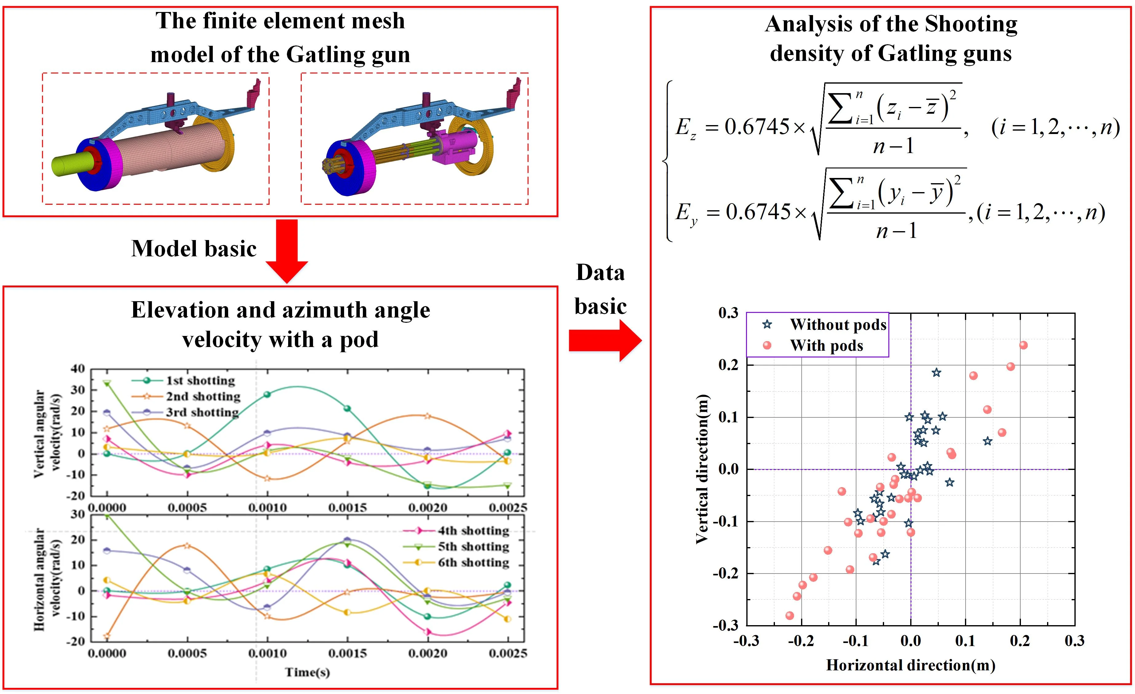
This paper conducted a numerical simulation study on the launch dynamics characteristics of Gatling guns under different conditions based on the nonlinear launch dynamics theory of artillery. A finite element mesh model of the Gatling gun was established, and combined with numerical simulation results, displacement cloud maps of the recoil motion direction with and without pods, as well as muzzle disturbance angle displacement and velocity curves of the Gatling gun were plotted. Finally, based on the six-degree-of-freedom rigid body ballistic equation of the projectile and the method of shooting density calculation, the firing densities of the Gatling gun under two scenarios were analyzed. This study reveals the launch dynamics characteristics of Gatling guns, providing effective references for the analysis of shooting vibration of Gatling weapon systems and even for the overall design and verification of weapons.

2. Artillery launch dynamics theory and numerical calculation of recoil process

In continuum mechanics, Lagrangian description and Eulerian description are two different forms of describing the deformation and response of continua. According to the firing scenario of Gatling guns, a system of equations is first used to describe the dynamic behavior of objects:

Considering the initial state $X_0$ of the object at time $t_0$, where the initial configuration is denoted as ${\mathrm{\Omega }}_0$ and the configuration boundary as $S_0$, after deformation, the state at time $t_1$ is represented by $x$, with the current configuration as ${\mathrm{\Omega }}_1$ and the configuration boundary as $S_1$. On the configuration ${\mathrm{\Omega }}_1$, the Cauchy stress tensor $\sigma \left(X,t\right)$, velocity vector $v\left(X,t\right)$, deformation rate tensor $F\left(X,t\right)$, and density $\rho \left(X,t\right)$ are chosen to obtain the discrete equations in Eq. (1). In the equation, $J$ represents the Jacobian matrix between the current and reference configurations; $\rho v_i^{\text{'}}$ denotes the particle inertial term; ${\epsilon }_{ij}$ and ${\sigma }_{ij}$ represent the strain and stress of the object, respectively, while $S$ is the material’s stiffness matrix. The geometric equation describes the relationship between the object’s deformation and displacement, the constitutive equation describes the relationship between the material’s strain and stress, and the boundary conditions define the force boundary ${\mathrm{\Gamma }}_{ti}$ and velocity boundary ${\mathrm{\Gamma }}_{vi}$.

Eq. (1) is known as the control equation in Lagrangian strong form. The finite element method cannot directly discretize the momentum equation. Multiplying the momentum conservation equation by the virtual velocity and integrating it within the current configuration ${\mathrm{\Omega }}_1$, considering the force boundary condition ${\mathrm{\Gamma }}_{ti}$, we obtain:

where, $n_s$ represents the dimension. When discretizing the control equation in the weak form using finite element method, the current domain ${\mathrm{\Omega }}_1$ is divided into multiple subdomains ${\mathrm{\Omega }}_e$, and the node coordinates in the current domain are denoted by $x_{Vi}$, where $V$ represents the nodal value, $i$ represents the component, $N_V$ represents interpolation function. The motion $x\left(X,t\right)$ and interpolated form of finite element displacement field and velocity variation can be expressed as:

Subsequently, based on the artillery launch dynamics theory, numerical calculations were conducted on the recoil force and recoil displacement of the Gatling gun under two conditions: without a pod and with a pod. The load curve is shown in Fig. 1(a), the calculated results of the recoil displacement and recoil force for the Gatling gun without a pod are shown in Fig. 1(b), and the calculated results of the recoil displacement and recoil force for the Gatling gun with a pod are shown in Fig. 1(c). In the case without a pod, the recoil displacement amplitudes of the first few shots are relatively large, and the amplitudes of the subsequent shots generally decrease gradually. Afterwards, the recoil displacement tends to stabilize in a cyclic pattern until shooting stops, returning to the initial position. As shown in Fig. 1(b), the variation trend of recoil force is similar to that of recoil displacement: the amplitudes of recoil force for the first few shots are relatively large, and then gradually decrease for the subsequent shots until the recoil force stabilizes in a cyclic pattern. After shooting stops, it decays back to the initial position. The maximum calculated recoil displacement is 9.47 mm, and the maximum recoil force is 30.98 kN.

Fig. 1Calculation results of the Gatling gun recoil

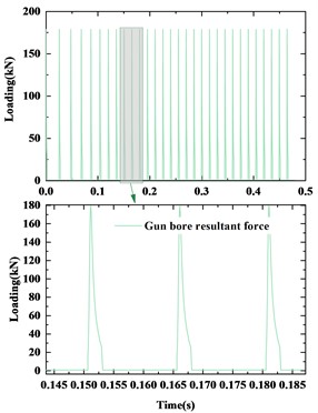
a) Load curve

b) Recoil displacement and recoil force curves

In the case with a pod, the maximum recoil displacement is quickly reached at the beginning of shooting. The amplitudes of the subsequent shots generally decrease gradually until the recoil displacement stabilizes in a cyclic pattern. As shown in Fig. 1(c), after shooting stops, it decays back to the initial position. The calculated maximum recoil displacement is 10.57 mm, and the maximum recoil force is 23.93 kN.

3. Numerical simulation of Gatling gun firing process

Firstly, based on the three-dimensional solid model of the Gatling gun, a finite element mesh model is established. The finite element mesh of the Gatling gun consists of 56164 elements, as shown in Fig. 2(a) and (b).

The spring element simplifies the buffer into a spring model, as shown in Fig. 2(c). When modeling the load, pre-tension forces are applied at the ends of the springs, as shown in Fig. 2(d). As shown in Fig. 2(f), the corresponding loads are applied when each barrel rotates to the firing position, with zero load during the intermediate period without chamber pressure. Rotational angular displacement is set for the connection part of the barrels, rotating counterclockwise when viewed from the gun’s tail, as shown in Fig. 2(g). The corresponding rotational angular displacement curve is determined based on the rules of the climbing and steady firing speeds, as shown in Fig. 2(e). The degrees of freedom other than the recoil direction at the bearing near the muzzle of the Gatling gun are constrained, as shown in Fig. 2(h). Additionally, the end faces of the brackets connected by the springs are fully constrained, as shown in Fig. 2(i). The end faces of entire mounting bracket connecting the Gatling gun with pod are fully constrained, as shown in Fig. 2(j).

Above the dashed line in Fig. 3 is the finite element simulation results of the Gatling gun without a pod, showing the displacement cloud maps of the recoil motion direction at the beginning of firing the first three shots and at the maximum recoil moment. Below the dashed line in Fig. 3 is the finite element simulation results of the Gatling gun with a pod, also showing the displacement cloud maps of the recoil motion direction at the beginning of firing the first three shots and at the maximum recoil moment.

Fig. 2The finite element mesh model of the Gatling gun with loads and boundary conditions: a) overall model, b) internal structure, c) spring elements, d) application of spring pre-tension forces, e) rotational angular displacement curve, f) loading conditions at the rear of the barrels, g) setting of rotational conditions at the barrel connection point, h) boundary conditions near the muzzle bearing, i) fixation at the tail bracket, j) fixed constraint boundary conditions

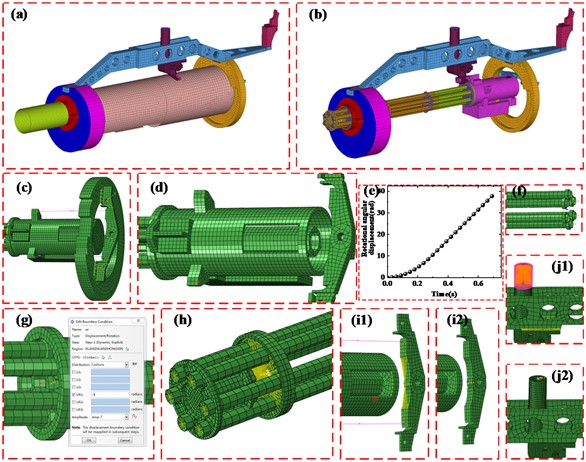
Fig. 3Cloud map of recoil motion direction displacement for the first three shots of the Gatling gun

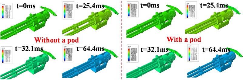
Fig. 4(a) and (b) show the partial muzzle disturbance simulation results of the Gatling gun without a pod for the first six shots from the beginning of firing to the moment of exiting the muzzle. Fig. 4(c) and (d) show the partial muzzle disturbance simulation results of the Gatling gun with a pod for the first six shots from the beginning of firing to the moment of exiting the muzzle.

4. Analysis of the shooting density of Gatling guns

By substituting the expressions for all forces and torques acting on the projectile into the general equation of rigid body motion of the projectile, the specific form of the projectile’s six-degree-of-freedom rigid body motion equation can be obtained, which is commonly referred to as the 6D equation. Let the ballistic coordinate system be $O{x}_2{y}_2{z}_2$. The ballistic coordinate system is a moving coordinate system with an angular velocity of $\mathrm{\Omega }$. Let the components of the vector $F$ of the external force along the axes of the ballistic coordinate system be $F_{x2}$, $F_{x2}$, $F_{x2}$ respectively. $M$ is the torque acting on the center of mass of the projectile by the external force:

Fig. 4Simulation results of muzzle disturbance for the first six shots of the Gatling gun

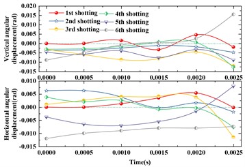
a) Elevation and azimuth angle displacement without a pod

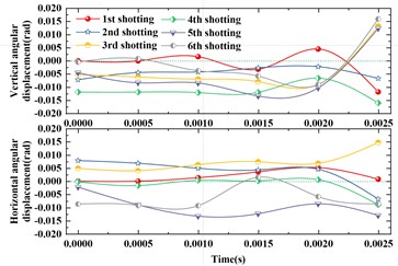
b) Elevation and azimuth angle displacement with a pod

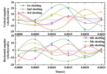
c) Elevation and azimuth angle velocity without a pod

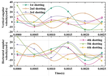
d) Elevation and azimuth angle velocity with a pod

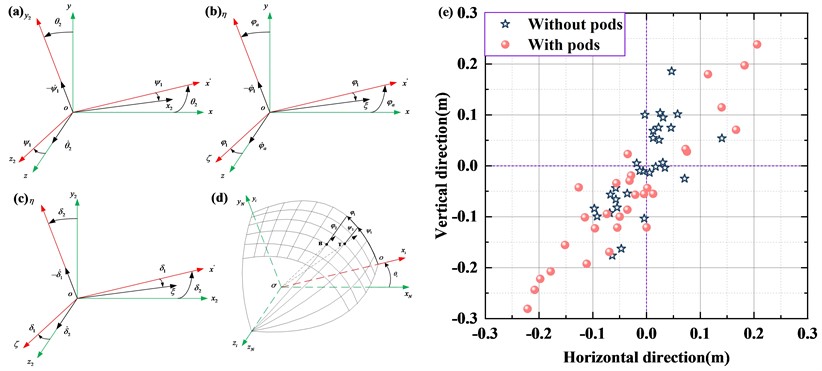
Simultaneously, the relationship between the ballistic coordinate system and the reference coordinate system $oxyz$ is shown in Fig. 5(a). The relationship between the projectile axis coordinate system $o\xi \eta \varsigma$ and the ground coordinate system is shown in Fig. 5(b). The relationship between the projectile axis coordinate system $o\xi \eta \varsigma$ and the velocity coordinate system is shown in Fig. 5(c). The specific spatial and physical meanings of the initial disturbance elements of the external ballistic trajectory are shown in Fig. 5(d). According to the calculation method of shooting density:

where, $E_z$ represents the azimuthal median deviation, $z_i$ represents the azimuthal scatter coordinate, $\stackrel{-}{z}$ represents the average value of azimuthal scatter coordinates, and $n$ represents the total number of projectiles. Similary, $E_y$ represents the vertical median deviation, $y_i$ represents the vertical scatter coordinate, $\stackrel{-}{y}$ represents the average value of vertical scatter coordinates.

The simulated results of the impact points in the elevation and azimuth directions at 50 meters are shown in Fig. 5(e). For the Gatling gun without a pod, the vertical elevation firing density is 1.1553 mrad, and the azimuth firing density is 0.7174 mrad; with a pod, the vertical elevation firing density is 1.7221 mrad, and the azimuth firing density is 1.5462 mrad.

Fig. 5Diagram of coordinate systems and calculation results: a) velocity coordinate system and ground coordinate system; b) projectile axis coordinate system and ground coordinate system; c) projectile axis coordinate system and velocity coordinate system; d) physical interpretation diagram of spatial initial disturbance of the projectile; e) calculation results of impact points for gatling guns without a pod and with a pod

5. Conclusions

This paper conducted a numerical simulation study on the dynamic launching characteristics of Gatling guns based on the theory of nonlinear artillery launch dynamics, and obtained the following important conclusions: Although the maximum recoil force with a pod is smaller than that without a pod, the results of horizontal angle and angular displacement for the first six shots show that the muzzle disturbance with a pod is more pronounced; at the same time, the recoil displacement with a pod is greater than that without a pod, and the calculation results of impact points for Gatling guns show that the firing density results with a pod are worse than those without a pod.

References

-
J. Xu and Z. Yang, “Structural multi-solution optimization and dynamics analysis of the main roller shaft of bolt,” in 2021 International Conference on Machine Learning and Intelligent Systems Engineering (MLISE), pp. 526–529, Jul. 2021, https://doi.org/10.1109/mlise54096.2021.00109
Y. Gao, Y. C. Bo, Z. Yang, and P. J. Zhang, “Movement dynamics analysis and optimization for external powered gatling gun,” Applied Mechanics and Materials, Vol. 488-489, pp. 951–954, Jan. 2014, https://doi.org/10.4028/www.scientific.net/amm.488-489.951
T. Li, R. L. Wang, and L. H. Liu, “dynamic simulation analysis of gatling gun based on virtual proto model,” Advanced Materials Research, Vol. 479-481, pp. 748–751, Feb. 2012, https://doi.org/10.4028/www.scientific.net/amr.479-481.748
M. Celik, Ü. Mercimek, and S. Kadıoğlu, “Shock failure analysis of metallic structures by using strain energy density method,” The Journal of Strain Analysis for Engineering Design, Vol. 49, No. 7, pp. 501–509, 2014, https://doi.org/10.1177/030932471453353
Ü. Mercimek, “Shock failure analysis of military equipments by using strain energy density,” Middle East Technical University, 2010.
About this article
This research was financially supported by the “China National Postdoctoral Program for Innovative Talents” [Grant No. BX20230493], the National Natural Science Foundation of China” [Grant No. 52305155], the “Jiangsu Province Natural Science Foundation” [Grant No. BK20230904], the “Jiangsu Province Excellent Postdoctoral Program” [Grant No. 2023ZB317].
The datasets generated during and/or analyzed during the current study are available from the corresponding author on reasonable request.
The authors declare that they have no conflict of interest.