Rolling bearing fault analysis based on variational mode decomposition and multiscale arrangement entropy

1. Introduction

Rolling bearings in machine tools and other equipment play an important role, which carries the main shaft of equipment, its operating status in a large extent affects the efficiency of equipment, so the bearings should maintain a better reliability. However, since the working characteristics of machine tools and other equipment, there are frequent startups, sudden changes in load, unstable rotation speeds and other working conditions, which will inevitably lead to bearing wear, cracks, gluing and other forms of failure occur, changes in the form of bearing structure will inevitably be expressed in the form of vibration signals [1]. Therefore, timely and accurate judgments of bearing faults through fault vibration signals [2] are essential for the stable operation of equipment [3-4].

Because of the complexity of the bearing conditions, it makes the fault characterization difficult [5]. In recent years, for the extraction of rolling bearing fault characteristics, the main methods used are Fourier transform, wavelet transform analysis, empirical mode decomposition (EMD) and variational mode decomposition (VMD), etc. [6]. Since the high requirements of wavelet basis function selection during signal decomposition, if the selected function cannot be adaptively decomposed, it will lead to a decrease in the accuracy of the studied results [7]. A consequent improvement is the method with adaptive decomposition of the signal – EMD. The signal is decomposed into multiple intrinsic modal components by EMD, and unlike wavelet analysis, the basis functions do not have to be chosen first, which gives EMD an advantage in dealing with nonlinear signals [8]. But EMD also has drawbacks, such as the presence of end-point effects and modal aliasing. The emergence of VMD addresses the shortcomings that existed in EMD. In 2014, a non-recursive, adaptive method for decomposing signals was proposed by Dragomiretskiy [9], the optimal center frequency and bandwidth of the decomposed modes are achieved with the help of the number of modes to be decomposed, i.e., the original signal is divided so that intrinsic modal function (IMF) are obtained for each of the $K$ frequencies. The shortcomings of EMD, such as the endpoint effect, are well addressed by selecting the value of $K$ in the VMD. From a mathematical point of view, VMD has a solid mathematical foundation [10]. The component decomposition capability possessed by the VMD is well demonstrated when feature extraction is performed on fault signals generated by bearing vibration: 1) The number of modal decompositions of bearing fault vibration signals can be determined adaptively depending on the actual situation; 2) With the Wiener filtering property possessed by the VMD, the noise can be strongly suppressed. Junzhong Xia et al. effectively extracted the fault features of bearings by VMD, and fully demonstrated that VMD could avoid the emergence of modal aliasing and other related problems when using EMD for feature extraction; Jie Shi et al. combined methods such as VMD and deep learning to successfully extract and analyze the fault characteristics of bearings [11], [12]. Luyang Jing et al. attempted to study the different performance of features by feeding raw, spectral, and combined time-frequency data into CNN [13]. Wei Zhang et al. proposed an end-to-end CNN framework without denoising preprocessing for studying bearing faults [14]. But there is no generalized method that can be applied to different bearings, and it is not easy to choose the right CNN framework and train parameters, and which mainly depends on human experience, so it is more time-consuming.

Bandt proposed Permutation Entropy (PE) [15], which can detect and quantitatively characterize the randomness possessed by time series. PE is a nonlinear metric. When the signal undergoes random changes, the signal can be detected and described by utilizing the characteristics of PE such as high sensitivity, strong noise elimination ability, and relatively simple and fast calculation. When quantifying rolling bearing fault signals in industrial machinery gearboxes, PE is used to provide timely feedback on bearing fault signal characteristics [16]. So based on the different PE values obtained, the health of the bearing can be determined. For example, an increase in the PE value indicates an increase in rolling bearing failures; a smaller PE value indicates better rolling bearing health. The variation of PE value directly reflects the failure condition of rolling bearings [17].

Aziz and other researchers were the first to elaborate on MPE concept in 2005. MPE effectively overcomes the drawback that PE can only measure the complexity of time series on a single scale. MPE can coarsely coarse-grain the time series so that different PE values can be obtained at multiple time scales. It can quantitatively analyze and comprehensively reflect the diversity and complexity, instantaneous changes in situation and magnitude of signals. In addition, MPE is more robust compared to PE [18-20]. Because there are complex structures in industrial machinery gearboxes, the information fed back by the signals generated by vibration is not only reflected in a single scale, but is fed back and reflected in multiple scales, so the vibration signals in industrial machinery gearboxes need to be analyzed in multiple scales. Peng Chen et al. improved MPE when it was used for fault diagnosis. Because the location of the fault and the type of fault are different, the feedback information is also different, this improvement can analyze the feedback information in a timely manner, which improves the correct rate of detection and diagnosis. Che Chang et al. constructed a neural network prediction model in their study, which was also based on MPE and long and short-term memory, and this study effectively reduced the probability of error in detection. Yanhe Xu et al. proposed a hybrid fault diagnosis method for rotating machinery based on variational mode decomposition energy entropy (VMD-EE) and transfer learning (TL), and the diagnostic results showed the accuracy and robustness of the proposed method [21]. Bearing fault diagnosis based on the classification of patterns of permutation entropy was proposed by Mantas Landauskas et al., and the validity of the method was verified by computational experiments [22]. Amir Eshaghi Chaleshtori et al. proposed a novel fault detection method for high-dimensional data, which significantly improved the accuracy of fault diagnosis using the weighted principal component analysis techniques and Gaussian mixture model [23]. Qing Li made the first attempt to combine asymmetric penalty regularization and SVD penalty regularization outside the sparse regularization and SLRM frameworks [24]. However, these methods have some disadvantages, such as slow extraction speed, low accuracy and poor feasibility. Gabriel Yuji Garoli et al. performed a sensitivity analysis by means of the Sobol index in order to assess which fault uncertainties can be ignored depending on the harmonic component [25]. In practical engineering applications, the actual operating data of the bearings and the parameters of the prediction model have a great deal of uncertainty, and if the uncertainty of the prediction results can be quantified, more information can be provided for maintenance decisions and risk assessment. Taylor proposed a more flexible model, quantized regression neural network (QRNN), in 2000; however, the shallow structure of QRNN lacks sufficient ability to simulate the complex temporal features of time series models [26]. Wen Chang Zhu et al. tested the dataset using RMT-PCA algorithm to verify the feasibility and validity of fusing feature index to assess bearing degradation under variable conditions. The statistical sample confidence was set to 95% and confidence interval was calculated to analyze the uncertainty of the fusion feature index. Under the premise of ensuring higher coverage, the narrower width indicates the better confidence interval effect and the less uncertainty in the assessment results. However, he did not consider whether the variation of the parameters had a significant effect on the reliability of the bearing assessment capability, and did not consider the uncertainty of the assessment results of the fusion characterization index when the parameters were varied [27].

During sound data acquisition for experiments such as load up/down for the start-up test of the Lianghekou No. 2 turbine unit, we analyzed the acquired sound data in terms of RMS, spectrum, and acoustic spectrogram. The neural network was chosen as an auxiliary means to enter the sound spectrogram as a training sample into the neural network input layer to obtain the sound pattern features, which were accessed into the clustering model to realize the classification, and to realize the classification scoring of the test samples [28]. In the process of anomaly detection of turbine operation status, we extracted the features of sound signals based on MobileFaceNet neural network. The improved Gaussian mixture model (i-GMM) was constructed using feature vectors and anomaly detection was performed on test samples. Validation of the effectiveness of the i-GMM model anomaly detection method was able to reach 100 % based on the bearing dataset [29]. In rolling bearing failure test signal analysis, we used a feature extraction method based on VMD and MPE to measure signal regularity and detect weak variations, which can more accurately diagnose different fault modes, different fault sizes, and different operating states of rolling bearings [30].

From the above analysis, for addressing limitations of analyzing fault signals separately for VMD and MPE, these two methods are combined to extract fault features from the vibration signals of rolling bearings in industrial machinery gearboxes, support vector machine (SVM) and $K$-nearest neighbor Algorithm (KNN) are innovatively used to identify and classify the intrinsic modal components and this method is very effective in analyzing the data. The experimental results also show that this method can effectively diagnose the type of rolling bearing faults in industrial machinery gearboxes. This method can overcome the disadvantages of the previous methods, for example, it can effectively improve the extraction speed, accuracy and feasibility.

2. Variational mode decomposition

Since Dragomiretskiy proposed the VMD algorithm in 2014, its application in fault diagnosis of rolling bearings has received increasing attention. Because the VMD algorithm can decompose the vibration fault signals of rolling bearings, it can decompose the complex fault signals into $K$ signal components with amplitude and frequency modulation. The $K$ value needs to be pre-set [31]. If a suitable value of $K$ is selected in the VMD algorithm, the modal aliasing and endpoint effect phenomena occurring in the EMD algorithm can be effectively suppressed by VMD. In essence, the method used for VMD denoising is Wiener filtering, so better denoising results can be obtained. Fundamentally, VMD is constructed and solved for variational problems. The VMD rationale works as follows:

1) Construction of variational problems.

The gearbox gear rolling bearing fault signal $f\left(t\right)$ is first decomposed into $K$ modal functions$\mathrm{}{u}_k$, which can be obtained by the following formulas:

where: ${\phi }_k\left(t\right)$ is the phase and is a non-decreasing function, ${\phi }_k^{\text{'}}\left(t\right)\ge 0$; the envelope is non-negative, $A_k\left(t\right)\ge 0$; the instantaneous frequency ${\omega }_k\left(t\right)={\phi }_k^{\mathrm{\text{'}}}\left(t\right)$ and the envelope $A_k\left(t\right)$ are slowly varying for the phase ${\phi }_k\left(t\right)$.

The $K$ modal components have a certain bandwidth frequency, and in order to obtain these modal components, the Hilbert transform of each modal function $u_k$ is required to obtain the marginal spectrum; the central frequency of each modal analytical signal is then mixed and predicted so that the spectrum of each mode can be modulated to the corresponding fundamental band; finally, the square $L^2$ norm of the analytical signal is computed to estimate the bandwidth of the signal for each mode; and the resulting variational problem is constructed as follows:

where: $\delta \left(t\right)$ is the impulse function; $\left\{u_k\right\}=\left\{u_1,u_2,\dots ,u_k\right\}$ and $\left\{{\omega }_k\right\}=\left\{{\omega }_1,{\omega }_2,\dots ,{\omega }_k\right\}$ are the $K$ components and the center frequency of each component obtained after decomposition, respectively.

2) Solution of variational problems.

To solve the constructed variational problem, the Lagrange multiplier operator and the quadratic penalty factor are introduced to obtain the extended Lagrange operator $L$ as follows:

where: $\alpha$ is the penalty factor parameter; $\lambda$ is the Lagrange multiplier.

The alternating direction multiplier algorithm is utilized for solving the above variational problem in the following steps:

Step 1. Initialize $\left\{{\widehat{u}}_k^1\right\}$, $\left\{{\omega }_k^1\right\}$, ${\widehat{\lambda }}^1$, $n$;

Step 2. Circulate $n=n+1$;

Step 3. When the condition $\omega \ge 0$ holds, the update of the generalized function ${\widehat{u}}_k$ is executed according to the cyclic program, the value taking of $u_k^{n+1}$ can be expressed as:

where: $\alpha$ is the penalty parameter; $\lambda$ is the Lagrange multiplier.

By using the Parseval theorem, the equation is transformed to the frequency domain:

The updated value is obtained after further transformation as follow:

where: ${\omega }_k$ is the center of gravity of the power spectrum of the modal function $u_k$. From Eq. (4), it can be seen that the Wiener filter is embedded in the VMD algorithm, which allows the VMD algorithm noise robustness to be enhanced.

Step 4. An update of the generalized function ${\omega }_k$, which can be expressed as:

The value taking of ${\omega }_k$ is transformed into the frequency domain:

The updated value is:

Step 5. An update of $\lambda$, it can be obtained by the following formulas:

where: $\tau$ is the noise tolerance limit.

Step 6. Repeat steps (2)-(5) until the iterative constraints are satisfied, which is formulated as follows:

End of iteration, output modal components.

3. Multi-scale permutation entropy

4. Bearing fault diagnosis analysis based on VMD and MPE

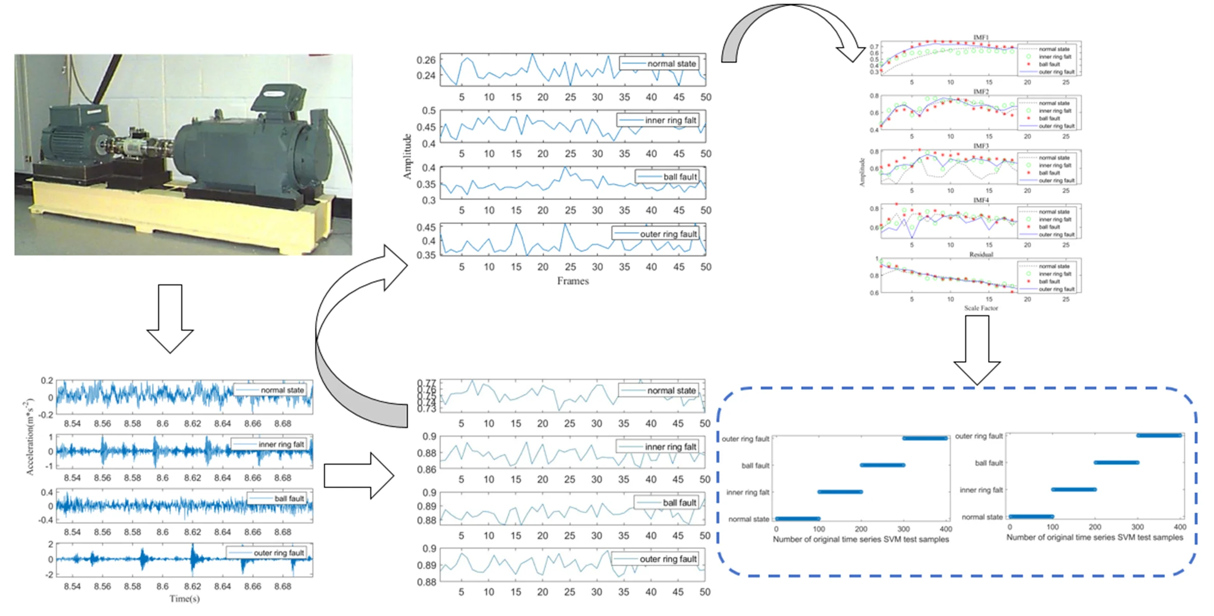
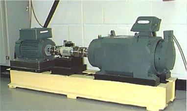
4.2. Bearing fault diagnosis analysis

In this paper, the bearing fault diagnosis analysis method based on VMD and MPE was applied to the bearing vibration experimental data analysis, the data were used in the bearing vibration related data provided by Case Western Reserve University Electrical Engineering Laboratory, Fig. 2 shows the test bench of the CWRU dataset, which consists of a 2 horsepower electric motor, a torque sensor and a power dynamometer. An acceleration sensor was placed above the bearing housing at the fan end and drive end of the motor to pick up the vibration acceleration signal of the faulty bearing, the vibration signals were acquired by a 16-channel data logger, power and speed were measured by torque transducer/translator. The faulty bearings were loaded into the test motor and the vibration acceleration signal data was recorded under 0, 1, 2 and 3 horsepower motor load operating conditions. 8 normal samples, 53 damaged samples of the outer ring, 23 damaged samples of the inner ring, and 11 damaged samples of the rolling element were obtained using this test bench. Each data file contains fan and drive end vibration data, as well as motor speed.

Fig. 1Fault diagnosis flowchart

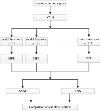
Fig. 2The test bench of the CWRU dataset

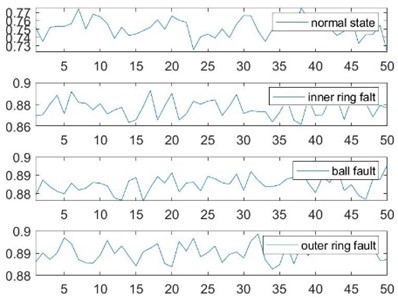
The model of the applied bearing was deep groove ball bearing SKF6205, with 9 rollers, fault diameter of 0.1778 mm, the power of the motor used for the test was 2 horsepower, the rotational speed was 1750 r/min, the sampling frequency was 12 kHz, and the length of the time series was 2048. Signals were collected for four states: normal state, inner ring fault, rolling body fault, and outer ring fault. The original time series display is shown in Fig. 3.

It can be seen from Fig. 3 that the three faulty vibration signals and normal vibration signals are somewhat different, the impulse frequency and amplitude have changed, but the difference is not particularly obvious.

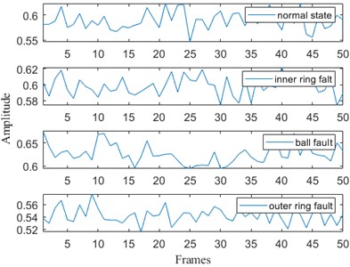
Fig. 4 shows the results of sample entropy calculation. The number of frames taken was 50, and the number of sampling points per frame was 2048. An average of 1.7322, 1.8995, 2.2384 and 1.4228 for the four states were obtained. The results were calculated by selecting different thresholds and the results were compared as shown in Table 1.

Fig. 3Original time series of the four states

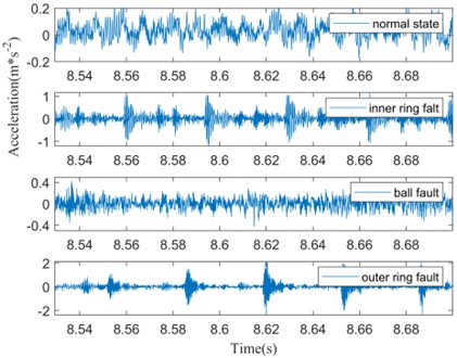
Fig. 4Sample entropy of the original time series

As analyzed above, the entropy value of the outer ring fault was reduced by 0.3094 compared to the normal state, which was due to the presence of periodic signals. Because the rotation signal of the rolling body was in an irregular form, the entropy value was enlarged. Therefore, faulty signals make it difficult to study and analyze the sample entropy. In this paper, the experimental data were analyzed for MPE, the embedding dimension $m=\text{6}$ and $\tau =\text{1}$ were selected to calculate the MPE value. When using VMD for decomposition, it is necessary to determine the value of the number of modal decompositions $K$. Too small a value of $K$ will lead to incomplete signals, while too large a value will lead to excessive decomposition, so $K=\text{4}$ was selected. The scale factor $s$ takes values generally greater than 12 and $s=\text{20}$ was selected.

Table 1Comparison of calculation results of different thresholds

	$R=$0.1	$R=$0.15	$R=$0.2	$R=$0.25
Normal status	0.5323	0.6764	0.7582	0.7639
Inner ring fault	0.6203	0.7891	0.8306	0.8161
Ball fault	0.6206	0.7966	0.8296	0.8185
Outer ring fault	0.6163	0.8015	0.8317	0.8252

The bearings studied were selected for four states of operation, namely: normal condition, inner ring failure, rolling element failure and outer ring failure. The original time series for different states were decomposed using the VMD method, the length of the time series was selected as 2048, and the sample entropy was extracted for a total of 50 time series, and the sample entropy averages of these 50-time series were obtained through the calculation, as shown in Fig. 5.

Fig. 5Permutation entropy calculation of the original time series

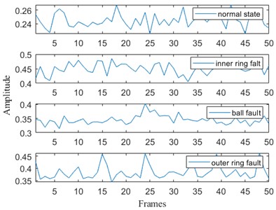
a) Mean values of IMF1: 0.2439, 0.3390, 0.3564 and 0.4150

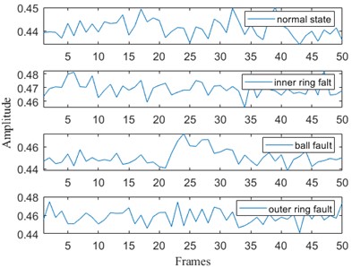
b) Mean values of IMF2: 0.3985, 0.4587, 0.4473 and 0.5014

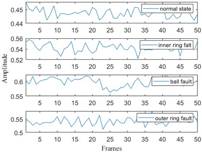
c) Mean values of IMF3: 0.4237, 0.5745, 0.5789 and 0.4902

d) Mean values of IMF4: 0.5384, 0.5396, 0.5006 and 0.5262

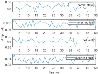
e) Mean values of residual: 0.7187, 0.8141, 0.8164 and 0.8616

As an example, one of the 50 time series was taken as an example to extract its multi-scale sample entropy, the scale factor $s$ took the value of 20, and the calculation results are shown in Fig. 6.

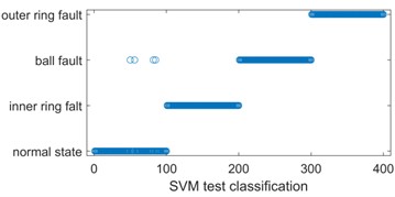
In order to test the diagnostic results, 100 time series were selected for each IMF of these four operating states, and the multi-scale sample entropy was extracted respectively, and a total of 400×20 samples obtained were labeled and inputted into SVM and KNN classifiers respectively, and the obtained results are shown in Fig. 7. It can be seen that three normal test samples were misclassified as rolling body faults when the SVM classification was performed.

Fig. 6Multi-scale permutation entropy for each IMF

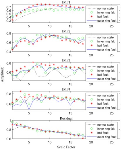
Fig. 7KNN and SVM classification comparison of IMF4 multi-scale permutation entropy

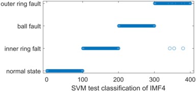
a) SVM test classification

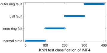
b) KNN test classification

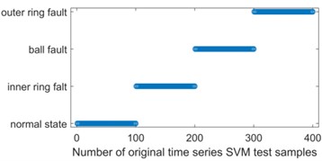
For further analyzing and comparing the accuracy of multi-scale sample entropy, each IMF of the four states was constructed as a 100×5 training sample, and a total of 400×5 samples were obtained, which were labeled and inputted into the SVM and KNN classifiers, respectively, and the obtained results are shown in Fig. 8. It can be seen that four normal test samples were misclassified as rolling body faults when the SVM classification was performed.

Fig. 8Comparison of sample entropy classification after original time series VMD decomposition

a) SVM test classification

b) KNN test classification

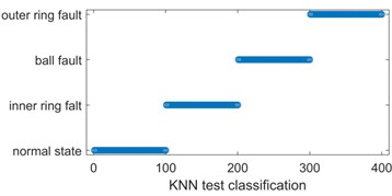
In order to further analyze and compare the accuracy of multi-scale sample entropy, each IMF of each state was constructed as a training sample constructed as 100×20, and finally 400×20 samples of the four states were labeled and inputted into SVM and KNN classifiers, respectively. This is shown in Fig. 9. According to the analysis of the Fig. 9, it can be seen that the use of both classification methods reached an accuracy rate of 100 %.

Fig. 9Comparison of multi-scale samples entropy classification for original time series

a) SVM test classification

b) KNN test classification

Data combinations 1 was tested for four conditions of a bearing with a loss diameter of 0.1778 mm: normal condition, inner ring failure, rolling element failure, and outer ring failure. In the test analysis, the prediction results of the IMF components and residuals were used to determine the attribution state by attribution degree calculation, and if the result belongs to whichever state the highest number of times, it is attributed to whichever state it belongs to. Specifically, as shown in Table 2, the accuracy of the VMD-synthesis method reached 100 % judgment.

Table 2Classification results for data combination 1

		Multi-scale MSE		Single scale SE
		KNN	SVM	KNN	SVM
VMD	IMF1	100 %	100 %	100 %	99 %
	IMF2	100 %	100 %
	IMF3	100 %	100 %
	IMF4	100 %	99 %
	Residual error	100 %	100 %
	Integrative	100 %	100 %	100 %	99 %
Original time series (OTS)		100 %	100 %

For further validation of the method proposed in this paper, data combination 2 tests were performed. The bearing load was 2 horsepower and the loss diameters were: 0.1778 mm, 0.3556 mm, 0.5334 mm, 0.7112 mm, respectively, and four operating conditions were tested and analyzed. As seen in Table 3, the test results show that there were a small number of sample false positives in the IMF4 and residuals, but the VMD-integrated determination method reached 100 % judgment.

Table 3Classification results for data combination 2

		Multi-scale MSE		Single scale SE
		KNN	SVM	KNN	SVM
VMD	IMF1	100 %	100 %	100 %	99 %
	IMF2	100 %	100 %
	IMF3	100 %	100 %
	IMF4	100 %	99 %
	Residual error	100 %	100 %
	Integrative	100 %	100 %	100 %	99 %
Original time series (OTS)		100 %	100 %

For further verification, data combination 3 was tested. The normal operations of the bearing under different loads were analyzed. It can be seen from Table 4 that the multi-scale sample entropy of the original time series was analyzed by SVM method, which obtained better test results; if the original time series were decomposed by VMD and the obtained sample entropy was analyzed by KNN method, it possessed better test results; the best test results were obtained when using VMD in combination with multi-scale sample entropy and inputting a KNN classifier for testing, and if the SVM method was used, the classification results were between the other two methods.

Table 4Classification results for data combination 3

		Multi-scale MSE		Single scale SE
		KNN	SVM	KNN	SVM
VMD	IMF1	100 %	100 %	100 %	99 %
	IMF2	100 %	100 %
	IMF3	100 %	100 %
	IMF4	100 %	99 %
	Residual error	93.26 %	85.32 %
	Integrative	100 %	100 %	100 %	99 %
Original time series (OTS)		100 %	100 %

5. Conclusions

In this paper, the vibration signals of four operating states of a rolling bearing with a loss diameter of 0.1778 mm were decomposed by VMD to obtain IMF functions, and the multi-scale sample entropy features of each IMF function were extracted. The constructed IMF training and test samples were fed into SVM and KNN classifiers for diagnostic test analysis, and the results were analyzed in conjunction with maximum imputation indexes. Subsequently, different combinations of data including different failure modes, different failure sizes and different operating conditions of rolling bearings were further tested and analyzed. The test results showed that based on multi-scale sample entropy, SVM and KNN classifiers, different fault modes, fault sizes and operating states of rolling bearings could be diagnosed more accurately, and it was concluded that this method could significantly improve the accuracy of the test. This method will be applied to more data combination tests in the future to improve the test and analysis methods, which can more accurately diagnose various failure conditions of rolling bearings with different parameters.