Abstract
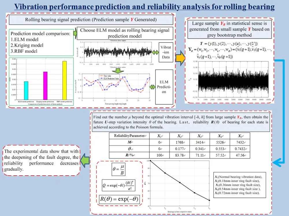
The bearing vibration signal is a rich dynamic symptom of bearing wear, and the vibration signal of rolling bearing presents chaotic characteristics. Input and output variables of vibration signal can be constructed through phase space reconstruction, the Input and output variables can be imported into the prediction model for prediction. The prediction accuracy of the extreme learning machine (ELM) model, Kriging model and RBF model are compared, the results show that ELM has higher accuracy, so ELM chaos model is used to predict the future vibration time series data, and the forecasting error can be obtained by comparing the prediction value with the actual values so as to verity the feasibility of the ELM model. The prediction results of the future state of the bearing are processed as the grey-bootstrap method, and the performance reliability prediction of the bearing is realized by the Poisson counting process. The experimental data show that with the deepening of the fault degree, the reliability performance decreases gradually. The reliability performance of the bearing without fault is 100 %, and the reliability performance is 47.56 % when the inner ring faulty size is 0.72 mm.
Highlights
- Rolling bearing prediction sample Y generated by ELM model
- Large sample YB in statistical sense is generated from small sample Y based on grey bootstrap method
- Reliability R(θ) of bearing for each state is achieved according to the Poisson formula
- The experimental data show that with the deepening of the fault degree, the reliability performance decreases gradually
1. Introduction
Rolling bearings are an important support for shafts and other rotating components, and their performance is vital for the normal equipment operation. As the core component of mechanical equipment, the vibration performance of rolling bearings is especially applied in the status assessment of high-precision equipment such as satellites and space shuttles. Therefore, the prediction of the rolling bearing vibration provides an important guarantee for the safe equipment operation.
Various factors are intertwined in the rolling bearing to cause their vibration performance nonlinear, these factors include: morphological characteristics of the roller contact surface and the viscosity-temperature effect of the lubricant [1]. The ununiformity of complex factors ultimately leads to the vibration performance extreme sensitivity. The method based on the chaotic phase space reconstruction theory allows accurate prediction of results of future rolling bearing vibration.
The phase space reconstruction made as the dynamic system method is the basis for analyzing chaotic time series. Since the 1980s, many domestic and foreign scholars have studied phase space reconstruction techniques. Among which the most widely used method is a delayed coordinate state space reconstruction theory proposed by Packard and Stewart [2]. Embedding-dimension and Delay-time parameters are used in phase-space reconstruction. The determination of these two parameters will affect the quality of phase space. Therefore, determining its value has very important theoretical and practical significance [3]. The commonly used methods to calculate the embedding dimension are saturation correlation dimension (GP), pseudo nearest neighbor method, Cao method, etc. [4-10]. Mutual information method, autocorrelation function method, and C-C method are used to calculate the delay time [11, 12].
Chaotic dynamics can be used to analyze time series with equal time intervals, the dynamic characteristics of chaotic systems can be indirectly obtained through the study of these time series, and these time series contain rich dynamic information. Extracting and using this information to study the characteristics of the system is one of the important aspects of chaos research. Many scholars have studied the chaotic dynamics of bearings, and the chaos performance of rolling bearing is studied in reference [13-16]. The authors [17] carried out a variable prediction research of rolling bearings. Professor Xia Xintao [18] used the Chaos-prediction method to predict bearing vibration time series, and the prediction error can be obtained through comparison and analysis between prediction value and true value.
The bearing reliability theory mainly involves the fatigue failure, and the establishment of models depends on the failure data greatly, which often ignores a large amount of evolutionary information of time series signals (such as vibration, temperature, friction torque, etc.) that promote the bearing degradation during its service life. By digging and extracting useful information of this type of time series, bearing performance prediction and reliability detection can be realized.
At present, bearing performance prediction and reliability research models are mostly based on the failure data or classical statistics, and there are relatively few research based on time series. In references [19, 20], it is recommended to apply a reliability prediction method based on the state information, the prediction model is used to accurately calculate the degradation index during the bearing service. The model establishment breaks through the limitations of traditional reliability large sample failure data. The authors [21] established an empirical probability density function for the friction torque parameters of aerospace bearings, the theory achieves accurate prediction for friction torque time series with the help of fuzzy sets. The authors [22] used nonlinear state estimation methods to effectively predict the temperature performance of gearbox bearings and accurately detect the operating state of gearboxes.
The prediction of bearing state is relatively single in the above research, and the prediction of bearing performance and reliability has not been carried out at the same time. In the process of bearing operation, an unexpected large vibration signal may appear, which may cause the peak value of time series, so monitoring and predicting the bearing performance is difficulty, the combination of performance prediction and reliability analysis has certain advantages, which can dig out the hidden information and discover the actual hidden danger in time. In the article, a chaotic prediction and reliability analysis of rolling bearing vibration time series is made. A chaos prediction model taken from the extreme learning machine (ELM) is constructed by solving parameters embedding dimension, delay time and using phase space reconstruction theory, and the chaotic prediction of rolling bearing vibration sequence is carried out. Secondly, a large number vibration variation sample is produced based on the grey-bootstrap-method. The Poisson counting theory is applied under a given threshold, and the corresponding variation intensity is obtained. According to the Poisson process, the predicted value of bearing reliability is obtained. The chaotic prediction and reliability analysis can be effectively applied to engineering practice.
2. Vibration prediction theory
2.1. Forecasting theory
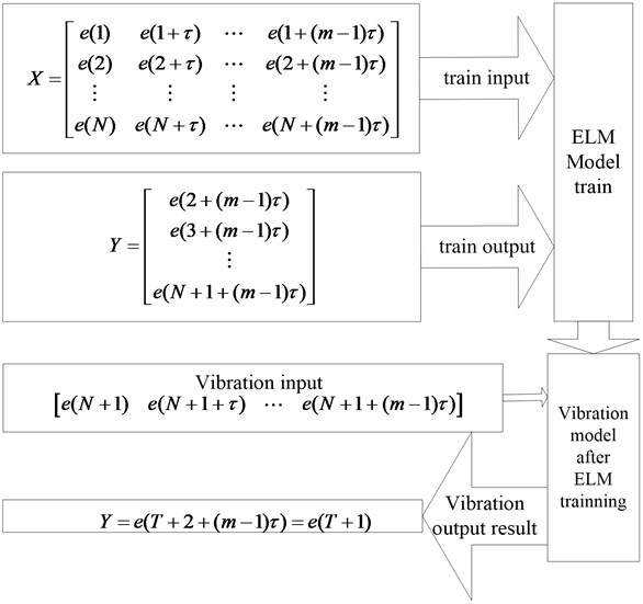
Suppose the rolling bearing vibration is given as X={e(i),i=1,2,⋯,T}, T is the number of time series. The matrices X and Y can be obtained using the delay coordinate method and are shown as follows:
where N=T-1-(m-1)τ, τ is delay time which is obtained by the autocorrelation function method, m is embedding-dimension which is calculated by the Cao-method.
According to the Takens theory, the reconstructed phase trajectory is dynamically equivalent to the original system in the homeomorphic sense. The rolling bearing vibration signal Y(i) can be predicted based on the point X(i) in the phase space, and the mapping function f is shown as follows, from which the next data point of time series can be gotten:
The own chaotic characteristics of the above prediction model, and the mapping function f has a non-linear structure. Traditional statistical methods such as auto-regression, moving average, and ARIMA are not suitable for solving it. Machine learning model ELM can establish non-linear mapping, which can act as mapping function to do such a prediction work, the specific prediction principle is shown in Fig. 1.
Fig. 1Chaos prediction theory
2.2. Delay time calculation theory
The autocorrelation function method is used to calculate a delay time parameter, which is constructed based on the linear correlation degree of two motion trajectory parameters at time t and t+τ. The autocorrelation function C(τ) of vibration series X=x1,x2,⋯,xn is shown as follows:
where ¯x is the mean value of the sample.
If the autocorrelation function shows significant attenuation trend with the growth of delay-time, the optimal delay time is equal to the time when the autocorrelation function reaches to 1-1/e times the initial value for the first time.
2.3. Cao method for embedding dimension
Cao Liangyue et al proposed the Cao method, which has the advantages of not-relying on the subjectivity and high calculation efficiency, let:
where, is phasor norm, is the th quantity of reconstructed phase space, where the embedding dimension is , is an integer greater than 1 and less than or equal to , and the sequence with the shortest distance from is .
The mean value of all is calculated using the above Eq. (5):
The embedding dimension is determined by observing the change of mean , along with , the change ratio is shown as follows:
When the change is stable, and the value of plus 1 at this time is the required embedding dimension.
The criteria for determining the stable change of are given below, the specific assessment process is as follows:
(1) is calculated as:
(2) An initial threshold is chosen according to the fluctuation of , here, , represents the average value of , and the subscript of the first is found, the value of is calculated:
(3) The values of , are reset as: , , where represents the average value of
(4) is taken when and and , embedding dimension is equal to .
Through the above criteria, a relatively objective evaluation can be made when tends to be stable, the embedding dimension calculation process is more scientific and rigorous.
2.4. ELM theory
ELM model is an algorithm proposed by Huang el al, which has its own advantages for training a single hidden layer feed-forward neural network. Its training model is shown in Fig. 2.
In Fig. 2, is the number of input-variables, shows the number of hidden layer neurons, represents the input variable, , represent the connection weight between the input variable and hidden layer neuron , represent the connection weight between output variable and hidden layer neuron , represent the threshold of hidden layer neuron, , represents the threshold of neuron in the output layer, represents the activation function of layered neurons, represents the activation function of output layer neurons.
Fig. 2ELM network structure
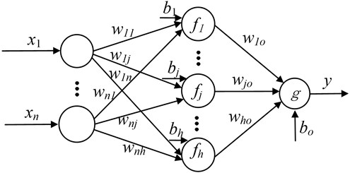
Its mathematical model is:
where, represents the output of output layer neurons .
If there are valid samples, when the output threshold is equal to 0, and the output neurons activation function is a linear activation function, then the Eq. (10) can be written as:
where, is the network output vector, represents the output weight vector, is the output matrix of hidden neurons, input weights and threshold matrix are randomly generated:
The expression of output weight vector is:
where, represents Moore-Penrose generalized inverse of output layer matrix is desired output. If , and , then the Moore-Penrose generalized inverse can be expressed as:
Putting Eq. (14) into Eq. (13), one can get:
The used hidden layer activation functions are Sigmoid function, Sin function, RBF function and Hardlim function.
2.5. Kriging model
The Kriging model can be expressed approximately as a sum of one random distribution function and one polynomial, as shown in Eq. (16):
where is an unknown Kriging model, is known as the two order regression function of , the global approximation model in the design space is provided, is the undetermined coefficient of regression function, its value can be estimated by the known response value, is a stochastic process, it is a local deviation on the basis of global simulation, and the expectation is 0, the variance is , the covariance matrix can be expressed as:
where R is the correlation matrix, represents the correlation function of any two sample points , , is the number of data in the sample. has a variety of functional forms can be selected, common correlation functions include cubic function, gauss function, linear function, spherical function, spline function and so on.
2.6. Radial basis function
Radial basis function (RBF for short) model is a kind of function which takes the Euclidean distance as the independent variable between the test point and the sample point.
RBF is one of the commonly used surrogate model, the basic form is as follows:
Basic function weight coefficient , and should meet the interpolation conditions:
where is the true value, is the prediction value, is the number of samples.
With:
where is radial function, common radial functions include Gaussian function, Multi-quadrics function, Reciprocal Multi-quadrics function, Thin-Plate spline function.
2.7. Accuracy evaluation method
Mean Squared Error (MSE), Root Mean Squared Error (RMSE) and Mean Absolute Error (MAE) indicators are used to calculate the prediction accuracy of the model, the expressions are:
where, represent the true value, represents the prediction value of the machine learning model, represents the number of test samples.
3. Reliability analysis theory
3.1. Grey-bootstrap method
According to the above prediction model, the vibration state information of bearing at the next step can be predicted, with the vector expressed as follows:
where, is the chaotic prediction data using the above ELM model, is the th data of data series, .
Using the above method, a number is randomly selected from using equal probability, the total selection number is equal to , so the bootstrap sample can be gotten, the above selection method is repeated times, and samples are obtained, the bootstrap sample is shown as follows:
where, represents the th bootstrap-sample, represents the total bootstrap-resample number, with:
where, and .
Based on the grey prediction model GM(1,1), supposing that the first-order accumulated generating operator for is as shown below:
The grey generated model can be described as the following differential equation:
where is time variable, and and are the undetermined coefficients.
Use the increment instead of differential, the above formula can be expressed as:
where, is equal to the unit time interval. Furthermore, the mean generated sequence vector is set as below:
Under the initial condition , the least-square-solution of the grey differential equation is shown as below:
where the determined coefficients and are shown:
with:
According to the inverse-accumulated generating, the th generated data are expressed as follows:
Therefore, generated data for rolling bearing vibration sample can be expressed as below:
where is the th produced data.
3.2. Poisson counting process
3.2.1. Counting process
Supposing that the generated-sequence (in Eq. (38)) for bearing’s future vibration signal has data over the vibration threshold , namely, there are data falling outside the interval of the best vibration performance, the variation intensity estimated value for is shown as follows:
Variation intensity refers to the frequency of the vibration amplitude for rolling bearing exceeding the optimal vibration performance interval, which is a vital characteristic parameter that affects the vibration variation process of the bearing operation, and it changes along with the different accuracy-threshold.
3.2.2. Rolling bearing reliability dynamic prediction
The Poisson counting process can be expressed as follows:
where stands for the time variable with , is the variation-intensity, is the failure event occurring number with , and is the probability of failure events occurring times. The reliability for occurring failure events can be obtained using the Poisson Counting process.
When solving the vibration performance reliability , the probability is equal to 0 when the product do not have a vibration failure, that is . And is the vibration performance reliability for the current time, namely the possibility of the vibration signal occurrence on the current generated sequence is within the optimal vibration interval . According to the above Eq. (40), the reliability can be described as:
where represents the probability for the rolling bearing to have within the optimal vibration during operation.
3.3. Modeling basic ideas
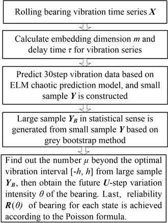
The theoretical modeling uses a variety of mathematical models such as ELM chaotic-prediction-model, grey-bootstrap method and Poisson counting process. The modeling method is shown in Fig. 3. The concrete steps are as follows:
Step 1. Based on the rolling bearing time series of the vibration performance, the embedding- dimension is obtained by the Cao-method, and the delay-time is obtained by the autocorrelation-method, so the phase-space-reconstruction can be realized based on the chaos theory.
Step 2. 30 step vibration data are predicted using the ELM chaotic prediction model, so the small sample can be constructed with the sample number of .
Step 3. A statistically large sample is generated from a small sample based on the grey-bootstrap method, so the Poisson count and bearing vibration variation strength can be easily gotten.
Step 4. Under the given vibration threshold , the number is found out beyond the optimal vibration interval from the large sample , and then the future -step variation intensity of the bearing is acquired, then, the reliability of the bearing for each state in the future is obtained according to the Poisson counting formula.
Fig. 3Vibration prediction and reliability analysis
4. Vibration analysis for rolling bearing
4.1. Vibration test data
The data used in this paper for experimental validation were provided by the Case Western Reserve University (CWRU), Cleveland, Ohio, USA [23]. As shown in Fig. 4, the test stand consists of an electronic motor, torque transducer, dynamometer, and control electronics. The bearing to be tested supports the motor shaft. The driving end bearing is SKF6205, and the fan end bearing is SKF6203. Acceleration sensors are placed above the bearing seat of the fan and the driving end of the motor to collect the vibration acceleration signal of the bearing.
Fig. 4Vibration experiment platform of rolling bearing
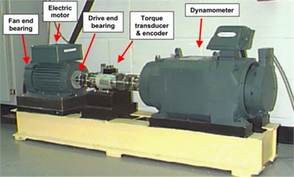
Fig. 5Layout of rolling bearing simulation experiment
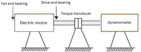
Vibration signal is collected by a 16-channel data logger, the power and speed are measured by a torque sensor. The test data are obtained by an acceleration sensor on the bearing at the drive end, and the rotation speed is 1796 rpm. Fig. 5 depicts a rolling bearing simulation experiment layout.
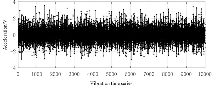
The above experimental platform is used to collect the rolling bearing vibration signal. The dynamic time data signals are collected as shown in Fig. 6 to 10. Fig. 6 to Fig. 10 respectively depicts the vibration data under normal bearing and four inner ring fault size.
Fig. 6Vibration data (normal bearing)
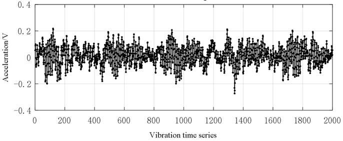
Fig. 7Vibration data (0.18 mm inner ring fault size)
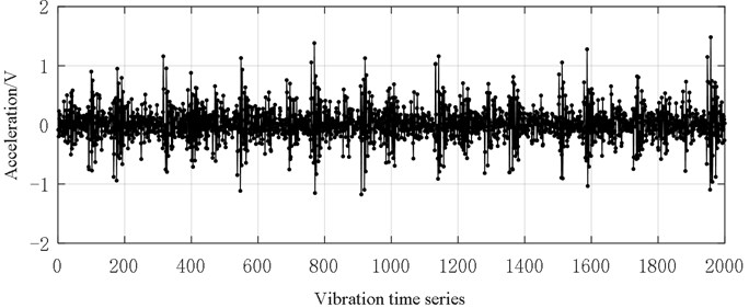
Fig. 8Vibration data (0.36 mm inner ring fault size)
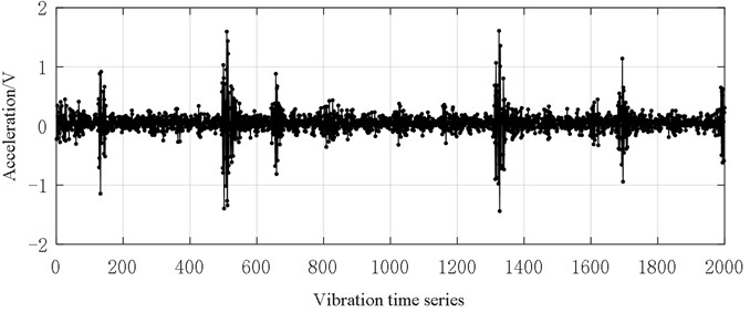
It can be seen from Figs. 6-10 that with the deepening of bearing failure, the overall vibration data of rolling bearings show an increasing trend. The vibration data of normal bearings is generally distributed between [–0.2, 0.2], and only a few data exceed this range. The bearing vibration data of the inner ring fault size of 0.18 mm is generally between [–1, 1], and data graph shows a similar saw-tooth shape. The bearing vibration data of the inner ring fault size of 0.36 mm is generally at [–1, 1]. these data near 500 series are significantly larger than other data. The bearing vibration data of the inner ring fault size of 0.54 mm is generally between [–2, 2], and the graph looks like a series of oval-shaped components. The bearing vibration data of the inner ring fault size of 0.72 mm is generally between [–4, 4], and the graph looks like a random distribution.
Fig. 9Vibration data (0.54 mm inner ring fault size)
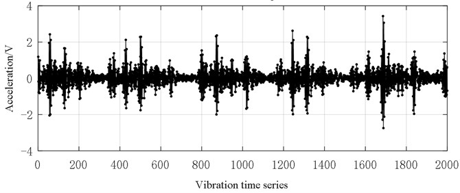
Fig. 10Vibration data (0.72 mm inner ring fault size)
4.2. Chaotic prediction with time series
The above mentioned bearing vibration time series are identified as (Normal bearing vibration data), (0.18 mm inner ring fault size), (0.36 mm inner ring fault size), (0.54 mm inner ring fault size), (0.72 mm inner ring fault size). The chaotic prediction method is used to predict these sequences, and the prediction step is 30, then the 2001-2030 original data are used to verify the accuracy and feasibility of five sequence prediction models.
Phase space parameter calculation: The auto-correlation method and Cao-method respectively have been used to acquire the delay-time and embedding-dimensions, and their results are shown in Table 1.
Table 1Phase space parameters of 5 series
Phase space parameter | |||||
Delay time | 4 | 1 | 1 | 1 | 1 |
Embedding dimension | 7 | 13 | 17 | 20 | 20 |
In order to compare the prediction accuracy of the three methods mentioned above, ELM model, Kriging model and RBF model are used to predict the next 30-steps of bearing vibration data, the comparison result between 30-steps chaotic prediction value and experimental value of above three methods are shown in Fig. 11. Among them, the red line means the experimental data, blue line means the ELM model predicted value, pink line means the Kriging model predicted value, and green line means the RBF model predicted value. The RMSE values for prediction error of three models mentioned above are shown as Fig. 12.
Fig. 11Prediction results comparison of the three methods
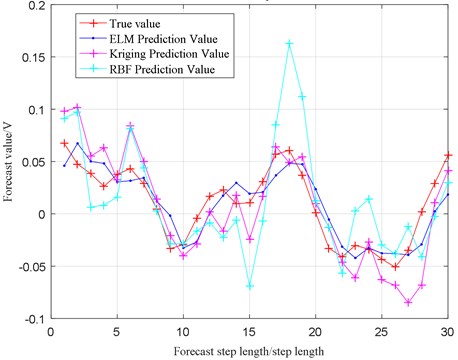
Fig. 12Prediction accuracy evaluation of the three methods (RMSE)
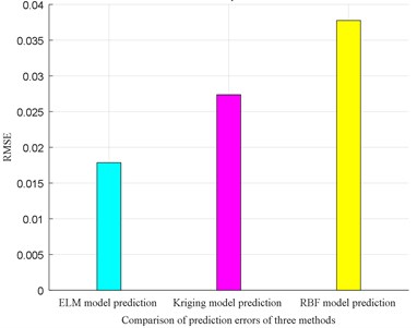
From Fig. 11 and Fig. 12, the message can be acquired that ELM model has the highest prediction accuracy compared with Kriging model and RBF model, so the ELM model is used to predict vibration signal for reliability analysis.
The determination of the phase-space parameters of the rolling bearing time series is the basis for its phase-space reconstruction, and it is required for preparing the chaotic prediction model. The comparison results between 30-step chaotic prediction value and experimental value for sequences data , , , , are shown in Figs. 13-17. Among them, the red line means the experimental data, and blue line means the predicted data.
From Fig. 13, the shape of the 30-step prediction result of the sequence is similar to the curve of the experimental result, the points that differ greatly from the original data are shown in step 1 and steps 19-21, where the maximum difference is only 0.0568 V.
From Fig. 14, the prediction results of the first 5 steps of the sequence are almost consistent with the original data. The steps 6, 13, 20, 22, 26, 28, 29 are significantly different from the original data, and the largest step is step 22 where the value is equal to 0.4152 V, the prediction results of other steps are almost consistent with the original data.
Fig. 13Vibration prediction data (X1)

Fig. 14Vibration prediction data (X2)
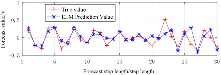
Fig. 15Vibration prediction data (X3)
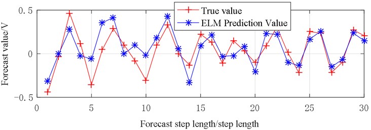
Fig. 16Vibration prediction data (X4)
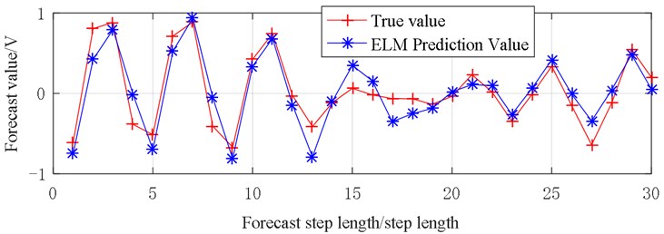
From Fig. 15, the prediction result of the sequence is relatively different from the original data, the largest step is step 10 equal to 0.2904 V, and the prediction error between steps 2, 13, 19, 26, 28, 29 and original data is relatively small.
From Fig. 16, the prediction results of the sequence are relatively similar to the original data. The fitting degree between prediction result line and the experimental result line at steps 1-12 and 19-30 are higher, only the prediction results of steps 12-18 are significantly different from the original data.
From Fig. 17, the prediction results of the sequence are similar to the original data, and the prediction result lines of steps 6-15 are almost identical to the original data, the change trend of the prediction lines of steps 15 to 30 is very similar to the original data, with a jagged jump between –2 and 2.
Fig. 17Vibration prediction data (X5)
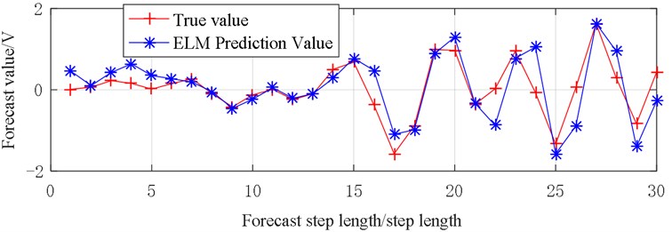
In order to scientifically evaluate the prediction accuracy, the RMSE value is used to calculate the prediction accuracy, as shown in Fig. 18.
Fig. 18Prediction accuracy evaluation (RMSE)
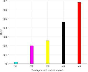
From Fig. 18, it is known that the RMSE evaluation value is small in each bearing state. When the inner ring fault size is 0.72 m, the RMSE value is approximately equal to 0.7 at the most.
In the 5 time series prediction of ELM chaotic prediction model, the difference between the predicted value and the experimental result is very small, and the two values maintain good consistency, that indicates that the prediction model is reliable.
4.3. Forecast results generated by grey-bootstrap method
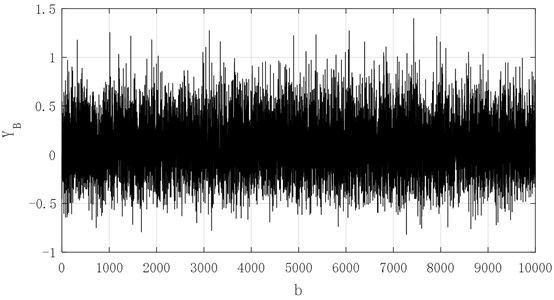
Now, the prediction results of the next 30 steps of each sequence are processed by grey-bootstrap method to simulate the large-scale generated data of the vibration performance for each state of the bearing in the next 30 steps. The generated data is doing Poisson count under the given threshold value, and then find the performance reliability of the bearing in the next 30 steps. In the grey-bootstrap generation, setting the sampling number 30 and repeated executions 10000, A large amount of generated-data in the next 30 steps for sequence , , , , is shown in Figs. 19-23.
Fig. 19Generated data of series X1 in future 30 steps
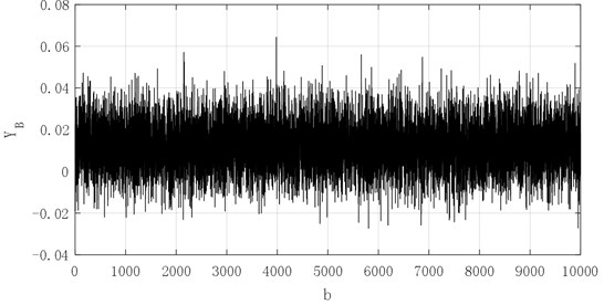
Fig. 20Generated data of series X2in future 30 steps
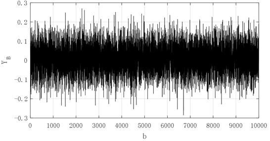
Fig. 21Generated data of series X3in future 30 steps
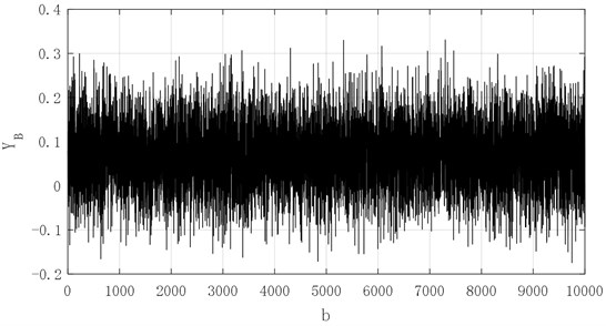
From the Figs. 19-23, the 10000 generated data simulated by grey-bootstrap-method has obvious randomness, and the corresponding value for sequences , , , and are concentrated in [–0.02, 0.06], [–0.2, 0.2], [–0.15, 0.3], [–0.4, 0.6] and [–0.5, 1]. The five sets of data show a non-linear increasing trend, which demonstrates that when the degree of failure deepens, the bearing vibration signal value gradually increases, and the inherent change law of the bearing vibration is closely related to the service life of bearing. Then, the evolution mechanism of performance reliability is determined and influenced.
Fig. 22Generated data of series X4in future 30 steps
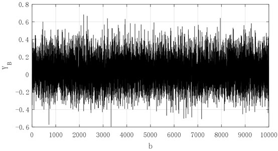
Fig. 23Generated data of series X5 in future 30 steps
4.4. Future state reliability assessment
The bearing vibration threshold 0.1 is set according to the generated data in Figs. 19-23, and the number of generated data is to be found for each sequence exceeding the vibration threshold , that is, the number that falls outside the optimal vibration interval [–0.1, 0.1] for the 10000 generated data of each sequence which can be calculated, so the variation intensity can also be obtained from the Eq. (39), then the reliability dynamic prediction result of the future 30 steps for each sequence can be calculated from Eq. (41). The results are shown in Table 2.
Table 2Number of μ exceeding vibration threshold h, variation intensity θ and performance reliability R
Reliability parameter | |||||
0 | 1768 | 3414 | 5526 | 7432 | |
0 | 0.177 | 0.341 | 0.553 | 0.7432 | |
/ % | 100 | 83.78 | 71.11 | 57.52 | 47.56 |
As it can be seen from Table 2, the data generated in the next 30 steps fall in the best vibration range for sequence , the variation intensity is 0, the reliability reaches 100 % that indicates that the bearing running state is relatively stable, no trace of bad behavior variation has occurred, and the state of maintaining the best vibration performance is very good.
In the sequence , the number of generated data in the next 30 steps that falls within the prescribed optimal vibration interval is 1768, the variation intensity is small and equal to 0.1768, and the reliability reaches 83.78 %, indicating that the bearing has a certain variation.
For the sequence , the number of generated data in the next 30 steps that falls within the prescribed optimal vibration interval is 3414, the variation intensity is relatively small and equal to 0.341, and the reliability is 71.11 %.
For the sequence , the number of generated data in the next 30 steps that falls within the specified optimal vibration interval is 5526, the variation intensity is more and equal to 0.553, and the reliability is 57.52 %.
For the sequence , the number of generated data in the next 30 steps that falls within the prescribed optimal vibration interval is 7432, the variation intensity is large and equal to 0.743, and the reliability is 47.56 %.
In order to describe the change of reliability intuitively, the change curve of the reliability parameter is shown in Fig. 24.
Fig. 24Change of reliability parameter R
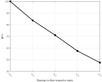
As shown in Fig. 24, as the degree of bearing failure deepens, the reliability gradually decreases from 100 % with zero-failure to 47.56 % when the inner ring failure size is 0.7112 mm.
As shown above, in the process of chaos prediction of bearing vibration time series, the prediction method of chaos prediction model based on ELM is accurate and reliable that meets the general prediction requirements of engineering practice. Combined with the grey-bootstrap method, the prediction value of each state sequence data in the next 30 steps is sampled and processed, and a large number of generated signals participated in bearing performance degradation is accurately simulated. The variation intensity obtained by counting process can effectively describe the variation degree of bearing, and can reveal the influence mechanism on the bearing state on the variation process of performance reliability in operation.
5. Conclusions
1) ELM model has the highest prediction accuracy compared with Kriging model and RBF model, so the ELM model is used to predict vibration signal for reliability analysis.
2) The chaotic prediction model based on the ELM is accurate and reliable. It can accurately predict the performance value of the future state of the bearing vibration time series. The predicted value and the true value can maintain a good consistency, which can be better applied to the engineering prediction.
3) The grey-bootstrap principle is integrated into the Poisson process, and a reliability prediction method is proposed based on the vibration time series, and it can ensure the performance reliability prediction of the future state of the bearing, and the variation characteristics of the variation intensity effectively reveal the state and its performance reliability variation process. The experimental data show that with the deepening of the fault degree, the reliability performance decreases gradually.
References
-
Xia Xin Tao, Xu Yong Zhi Modern Statistical Analysis of Variation of Rolling Bearing Performance. Science Press, Beijing, 2016.
-
Prokhorov M. D., Ponomarenko V. I., Karavaev A. S., et al. Reconstruction of time-delayed feedback systems from time series. Physica D, Vol. 203, 2005, p. 209-223.
-
Camplani Massimo, Cannas Barbara Role of embedding dimension and time delay in time series forecasting. IFAC Proceedings Volumes, Vol. 42, Issue 7, 2009, p. 316-320.
-
Qiu Huaxu, Huang Zhangyu, Zhu Hua Application of improved G-P method in time series study. Reconnaissance Science and Technology, Vol. 1, 2014, p. 53-54.
-
Adenan Nur Hamiza, Rani Mohd Salmi Md Noo Predicting time series data at floodplain area using chaos approach. Sains Malaysiana, Vol. 44, Issue 3, 2015, p. 463-471.
-
Small Michael, Tse C. K. Optimal embedding parameters: modeling paradigm. Physica D, Vol. 194, 2004, p. 283-296.
-
Maus A., Sprott J. C. Neural network method for determining embedding dimension of time series. Communications in Nonlinear Science and Numerical Simulation, Vol. 16, Issue 8, 2011, p. 3294-3302.
-
Meng Qing Fang, Zhangqiang, Pan Jin Feng New method for determining minimum embedding dimension based on four-order cumulant. Theory and Practice of System Engineering, Vol. 9, 2005, p. 83-88.
-
Sun Yun, Wang Ying, Meng Xiangfei, et al. Methodology of estimating the embedding dimension in chaos time series based on prediction performance of K-CV_GRNN. International Conference on Information Systems and Computer Aided Education, 2018.
-
Cao L. Practical method for determining the minimum embedding dimension of scalar time series. Physica D: Nonlinear Phenomena, Vol. 110, Issue 1, 1997, p. 43-50.
-
Fraser A. M., Swinney H. L. Independent coordinates for strange attractors from mutual information. Physicalreview A, Vol. 33, Issue 2, 1986, p. 1134.
-
Kim H. S., Eykholt R., Salas J. D. Nonlinear dynamics, delay times, and embedding windows. Physica D, Vol. 127, 1999, p. 48-60.
-
Long Chen, Xin Tao Xia, Hao Tian Zheng, Ming Qiu Chaotic dynamics of cage behavior in high-speed cylindrical roller bearing. Shock and Vibration, Vol. 2016, 2016, p. 9120505.
-
Zhang Shuqing, He Peng, Zuo Yige, Chen Rongfei, Zhang Yun, Liu Wan, Jiang Wanlu Study on characteristics of chaotic singular spectrum and applications in rolling bearing fault diagnosis. China Mechanical Engineering, Vol. 29, Issue 492, 2018, p. 16-22.
-
Li Zhaofei, Renxiaohong, Huang Chencheng Study on nonlinear hyper chaotic characteristics for vibration of rolling bearings. Bearing, Vol. 7, 2016, p. 54-60.
-
Xu Yong Zhi, Xia Xin Tao, Nan Xiang Dynamic analysis of robust test data on rolling bearing vibration based on chaos theory. Journal of Aerospace Power, Vol. 30, Issue 8, 2015, p. 1959-1965.
-
Pan Haiyang, Yang Yu, Zhengjinde, Cheng Junsheng Variable predictive model based RBF class discriminate method. Journal of Aerospace Power, Vol. 32, Issue 2, 2017, p. 500-506.
-
Xiaxintao, Chang Zhen, Li Yunfei Vibration performance prediction and reliability analysis for bearins. Journal of System Simulation, Vol. 30, Issue 4, 2018, p. 1390-1398.
-
Lihongkun, Zhang Zhixin, Li Xiugang, et al. Reliability prediction method based on state space model for rolling element bearing. Journal of Shanghai Jiaotong University (Science), Vol. 20, Issue 3, 2015, p. 317-321.
-
Xiao Wenrong, Cheng Wei, Zi Yangyang Support evidence statistics for operation reliability assessment using running state information and its application to rolling bearing. Mechanical System and Signal Processing, Vol. 60, Issues 61-11, 2015, p. 344-357.
-
Xia Xintao, Jia Chenhui, Wang Zhongyu Fuzzy prediction of rolling bearing friction torque using information poor system theory. Journal of Aerospace Power, Vol. 24, Issue 4, 2009, p. 945-950.
-
Li Dazhong, Chang Cheng, Xu Bingkun Wind turbine gearing temperature prediction based on sample optimization. Journal of System Simulation, Vol. 29, Issue 2, 2017, p. 374-380.
-
Chaozhong Guo, Lin Li, Yuanyuan Hu, Jihong Yan A deep learning based fault diagnosis method with hyperparameter optimization by using parallel computing. IEEE Access, Vol. 8, 2020, p. 131248-131256.
Cited by
About this article
This paper is supported by the National Natural Science Foundation of China, (No. U1804141), by the Program for Science and Technology Innovation Talents in Universities of Henan Province (No. 17HASTIT028), by the Key Science and Technology Research Project of the Henan Province (No. 212102210071) and by Educational commission of Henan province (No. 21A460037).

