A rolling bearing fault diagnosis method based on Compressive sensing and Local characteristic-scale decomposition

1. Introduction

Bearings are mechanical components that are the spindle point, and once bearing failure occurs, the machine cannot operate safely and the efficiency of the machine will also be reduced. The bearing of an operating machine is usually vibratory and its vibration signal contains a lot of state information. Therefore, the measurement and analysis of vibration signals generated by bearings can be used to identify and classify the fault state.

Fault diagnosis by vibration signal analysis is generally performed in the time domain, frequency domain or time-frequency domain. Statistical parameters have been often used to detect bearing faults in the time domain [1]-[2]. This type of method is relatively simple but it cannot identify the fault types with high precision. Especially, the roller bearing vibration signal has nonlinear and nonstationary characteristics so that it is insensitivity to diagnosis the roller bearing fault [3]. Frequency domain methods describe signals more clearly and it can reflect more details of fault degradation degree. Therefore, in recent years, the time-frequency analysis methods have been widely used [4]-[5]. These methods can provide the local characteristics of signals in both time domain and frequency domain. The time-frequency decomposition methods include empirical mode decomposition (EMD), local mean decomposition (LMD), and local characteristic-scale decomposition (LCD) and so on.

The EMD method proposed by Huang et al is an adaptive decomposition method [6]. This method can effectively decompose the local feature of the signal into several components, and has the ability to process

complex nonlinear and nonstationary signal. So it is widely used in fault diagnosis [7]-[8]. The envelope analysis method and EMD method are combined and applied to the fault diagnosis of roller bearings, and better analytic results are obtained [9]. However, owing to the EMD problems such as the over envelope, the owing envelope, mode mixing, and the end effect [10], the application effect of this method in practical engineering is affected to some degree.

The LMD method proposed by Smith [11] in 2005 is similar to the EMD method, and is also based on the inherent characteristic of vibration signal to decompose complex signals. Because of the use of the division operation to obtain the product function (PF) component, it can reduce the number of iterations and then reduce the end effect. At the same time, the effect of the LMD method overcoming the over envelope and the owing envelope is better than the EMD method [12]. This method can decompose the PF components which can be closely related to fault. In literature [13], by analyzing the spectrum of PF components, the characteristic information of fault frequency is extracted accurately. However, because the traditional LMD method has defects such as a poor ability to extract weak high frequency components, a large amount of iterative calculation, and the frequency confusion [14], it needs to be further optimized.

The LCD method is a new adaptive time-frequency analysis method based on intrinsic time-scale decomposition proposed by Yang et al. [15]. This method utilizes piecewise linear transformation to obtain the baseline signal, which can avoid the EMD problems such as over envelope and owing envelope etc. It can also reduce computation complexity of EMD and LMD. The iteration number is relatively small and the speed is fast, so it is more suitable for online real-time monitoring and processing of signals [16]. This new time-frequency analysis method has been mainly employed in vibration signal processing and fault diagnosis and has made some achievements in the past few years.

On the other hand, the complex and nonstationary vibration data with a large amount of noise make the failure detection very challenging, especially at the early stage. By means of appropriate vibration signal processing, it is feasible to detect the failure to evaluate the operational conditions qualitatively and quantitatively.

The measured vibration signals often contain noises, which may arise due to sensor imperfection, poor surrounding environment, or communication errors. Useful features information is therefore usually too weak to be distinguished. Removing such noises is of great benefit in successive applications.

There are many denoising methods include singular value decomposition [17], wavelet analysis [18], etc. For the SVD method, in order to discriminate against noise, it decomposes the column space of observation matrix into a dominant and a subordinate part, revealing which of its subspaces can be attributed to the noise-free signal and which can be attributed to the noise. It is often assumed that these two subspaces are orthogonal to each other, which implies that signal and noise are independent. For image de-noising, the basic idea is to retain the energy in the signal subspace and discard the energy in the noise subspace. Denoising by wavelet methods has received much interest [19]-[20]. With wavelet transform, one can decompose the original signal into a smooth part (subband in terms of signal processing) and a detail part. For most signals, energy mainly distributes in the smooth subband, and energy in the detail subband is clustered on a few large wavelet coefficients, corresponding to the edge structure of original signal. In contrast, noise energy spreads over both the smooth subband and the detail subband. With orthonormal wavelet, white noise is also white in the transform domain.

These methods are based on the sampling theory that the sample frequency must be twice the maximum frequency to be analysed. This basic principle underlies the majority of digital signal processing applications such as audio, video, radio receivers, radar applications, medical devices and more. The theory indicates that a large amount of data must then be collected, creating an exceptional challenge for signal acquisition, transmission and processing. Compression of large-scale monitoring data to detect fault features directly from sparse samples is one way to address the challenges.

Compressive sensing (CS) that emerged in 2005-2006 [21-23] breeds a new method to extract impulse signal from heavy noises. The core theory of the CS model is the sparse representations/approximation. CS lies on the assumption that it is possible to reconstruct a sparse signal exactly from only a few samples, namely solving an underdetermined linear system of equations [24]. The application of CS on image de-noising [25] and speech enhancement [26]-[27] etc. had been studied since the CS theory appeared.

With the advancement of wireless sensors and communication technologies, it is now possible to monitor machines remotely. In this application, the use of compressive sensing is very useful because of its high accuracy and low computational cost due to de-noising during signal processing.

2. CS and LCD

2.1. CS

CS theory was newly presented in 2006 in the field of signal processing and has been used in various fields such as image de-noising and speech enhancement.

CS can be divided into two steps [11]. First, combining the sampling with compressing, $x$ original signal with the compressed signal by using an appropriate recovery algorithm.

The original signal $x\in R^N$ can be sampled as a compressed signal with reduced order $y\in R^M$ by following:

1

$y=\mathrm{\Phi }x,$

where $\mathrm{\Phi }\in {\mathrm{R}}^{M\times N}(M<N)$ is a compressive matrix.

According to linear algebra theory, Eq. (1) has infinite number of solutions and when $M<N$, we cannot recover the original signal $x$ uniquely from the compressed signal $y$. However, if the signal $x$ is sparse, i.e., there only has a few nonzero coefficients in $x$, it is possible to recover $x$ from $y$. Generally, the vibration signals should not be sparse, while they can be represented sparsely by some appropriate ways (e.g., orthogonal transformation).

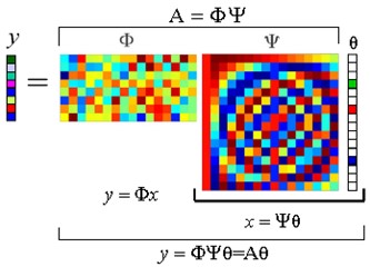
Using some orthogonal basis $\left\{{\psi }_i\right\}(i=1,N)$, we can expand $x\in R^N$ as:

2

$x={\sum }_{i=1}^N{\theta }_i{\psi }_i,$

where the coefficient ${\theta }_i=〈x,{\psi }_i〉={\psi }_i^{T}x$ and $\left\{{\psi }_i\right\}$ is an $N$-dimensional column vector. Expressing Eq. (2) in matrix form, we can get:

3

$x=\mathrm{\Psi }\mathrm{\Theta },$

where $\mathrm{\Psi }=[{\psi }_1,{\psi }_2,\cdots ,{\psi }_N]\in R^{M\times N}$ is called a dictionary matrix and $\mathrm{\Theta }={\{{\theta }_1,{\theta }_2,\cdots ,{\theta }_N\}}^T$ is a coefficient vector. Substituting Eq. (3) into Eq. (1), and denoting $A=\mathrm{\Phi }\mathrm{\Psi }$:

4

$y=\mathrm{\Phi }\mathrm{\Psi }\mathrm{\Theta }=A\mathrm{\Theta },$

where $A$ is called the measurement matrix.

Suppose that the coefficient vector $\mathrm{\Theta }$ is $k$-sparse on the basis $\mathrm{\Psi }$, i.e. there are $k$ nonzero elements in $\mathrm{\Theta }$. That is, unknowns in the above equation will be greatly reduced so that it is possible to recover $\mathrm{\Theta }$ from $y$.

We will choose the Orthogonal Matching Pursuit-OMP algorithm for signal recovery. Since $\mathrm{\Theta }$ has $k$ nonzero components, the vector $y=A\mathrm{\Theta }$ is a linear combination of $k$ columns from $A$. In the language of sparse approximation, we say that $y$ has an $k$-term reperesnetation over the dictionary $A$.

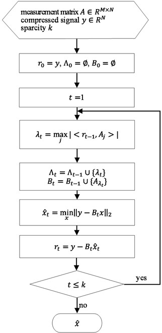
Therefore, sparse approximation algorithm can be used for recovering sparse signals. To identify the ideal signal $\mathrm{\Theta }$, we need to determine which columns of $A$ participate in the vector $y$. At each iteration, we choose the column of $A$ that is most strongly correlated with the remaining part of $y$. Then we subtract off its contribution to $y$ and iterate on the residual. After $k$ iterations, the algorithm will have identified the correct set of columns. The steps of OMP algorithm are as follows:

Input: measurement matrix $A\in R^{M\times N}$, compressed signal $y\in R^M$ (be obtained by Eq. (1)), the sparsity level of the signal $k$.

Initialization: the residual $r_0=y$, the index set ${\mathrm{\Lambda }}_0=\varnothing$, the matrix $B_0=\varnothing$.

FOR $t=1$; $t=t+1$; $t\le k$

Step 1: Find the index that solves the easy optimization problem ${\lambda }_t=\underset{j}{\max }\left|〈r_{t-1},A_j〉\right|$, where $A_j$ is $j$-th column of $A$.

If the maximum occurs for multiple indices, break the tie deterministically.

Step 2: Update the index set and matrix: ${\mathrm{\Lambda }}_t={\mathrm{\Lambda }}_{t-1}\cup \left\{{\lambda }_t\right\}$, $B_t=B_{t-1}\cup \left\{A_{{\lambda }_t}\right\}$

Step 3: Solve a least squares problem to obtain a new signal estimate: ${\widehat{x}}_t=\underset{x}{\min }{‖y-B_{t}x‖}_2$.

Step 4: Calculate the residual: $r_t=y-B_t{\widehat{x}}_t$.

END FOR

Output: An estimate ${\widehat{x}}_k$.

The flowchart of OMP algorithm for signal recovery is shown in Fig. 1.

Fig. 1The flowchart of OMP algorithm

2.2. LCD

Local Characteristic-Scale Decomposition (LCD) is a new adaptive time-frequency analysis method based on time-scale decomposition.

Theoretically, this method is of great interest in the field of vibration signal processing recently because it decomposes the signal into a space of orthogonal frequency basis, has the unique character of signal decomposition, has the excellent localization properties in both time and frequency domains simultaneously, and has a much superior signal decomposition rate and self-signal adaptation characteristics compared with existing signal decomposition methods, including empirical mode decomposition and local mean decomposition.

Once the signal decomposition is complete, the signal reconstruction can be done according to the requirements of the detailed problem. We give an iterative formula for the ignition of the intrinsic scale component (ISC) based on the principle of the LCD method. By decomposing any signal into a signal of different frequency, it is possible to extract information from the signal of sine or cosine exponential decay.

First of all, we define the ISC and consider the factors that affect the procedure and accuracy of the LCD method to obtain it.

2.2.1. ISC

To use the LCD method, we define the intrinsic scale component (ISC). The intrinsic scale component is a single-component signal expressed as instantaneous frequency that is physically meaningful based on local characteristic parameters of the extrema. The ISC must satisfy the following two conditions to have physical meaning.

1. For the data set, the marks of any two adjacent extrema are mutually different.

2. For the data set, the extrema are $L_k$, $k=1,\mathrm{}2,\mathrm{}\cdots ,\mathrm{}M$ with their respective corresponding moment ${\tau }_k$, $k=1,\mathrm{}2,\mathrm{}\cdots ,\mathrm{}M$. The section of line formed by connected any two maximum (minimum) extrema (${\tau }_k$, $X_k$), (${\tau }_{k+2}$, $X_{k+2}$) is between them. Therefore, we can obtain the corresponding moment ${\tau }_{k+1}$ of the maximum (minimum) extrema, and the function value is set to:

5

$H_{k+1}=L_k+\frac{{\tau }_{k+1}-{\tau }_k}{{\tau }_{k+2}-{\tau }_k}\left(L_{k+2}-L_k\right),$

of which the ratio to the relative maximum(minimum) extrema $L_{k+1}$ remains unchanged.

These two conditions ensure that there is a single mode between any two adjacent extrema of ISC, and the local curve (curve between extrema and adjacent zero point) approximate to the standard sine curve, so the instantaneous frequency has physical significance.

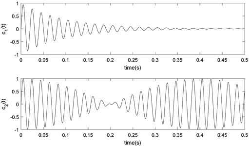
Fig. 2An example of ISC: c1t=e-10tsin⁡100πt, c2t=0.5sin⁡100πt+0.5sin⁡105πt

The two end points of the envelope (starting and ending points) are obtained by spline interpolation.

Note that the ISC of the difference is the one that should be passed over, but the modal analysis theory only includes a modal signal of some order (not necessarily difference).

The latter include vibration mode amplitude, natural frequency and damping of some order.

The angular mode order signals are independent of each other and decompose the signal into frequency orthogonal basis space. That is, the decomposition of the signal has uniqueness.

Fig. 2 shows an example of two functions that fit the conditions of the ISC. As you can see, the ISCs are functions of local symmetry up and down with respect to the zero axis.

2.2.2. Ignition-iteration formula for ISC calculations

The algorithm for decomposing the signal $x\left(t\right)$ using the LCD method is as follows.

Step 1: Calculate extreme points $L_k\mathrm{}(k=\mathrm{1,2},\cdots ,j)$ of the signal $x\left(t\right)$, and then calculate the fitting points:

6

$g_k=\frac{L_k+H_k}{2}.$

Step 2. On the basis of extending the endpoints in time series, use cubic spline function for fitting all $g_k$, and at last get the mean curve $B_{g_1}\left(t\right)$.

Step 3: Eliminate the mean curve $B_{g_1}\left(t\right)$ from the original signal:

7

$P_{11}\left(t\right)=x\left(t\right)-B_{g_1}\left(t\right).$

Eq. (7) is called the “decreasing average” process.

Step 4: Judge whether $P_{11}\left(t\right)$ meets the ISC conditions or not. If it is satisfying, take $P_{11}\left(t\right)$ as the first ISC, signed as ${\mathrm{I}\mathrm{S}\mathrm{C}}_1\left(t\right)$. If not, take $P_{11}\left(t\right)$ as the original signal and repeat steps (1)-(3):

8

$P_{12}\left(t\right)=P_{11}\left(t\right)-B_{g_2}\left(t\right),$

9

$P_{13}\left(t\right)=P_{12}\left(t\right)-B_{g_3}\left(t\right),$

$⋮$

10

$P_{1k_1}\left(t\right)=P_{1k_1-1}\left(t\right)-B_{g_{k_1}}\left(t\right).$

And then cycle $k_1$ times until $P_{{1k}_1}$ meets the ISC contitions, thus $P_{{1k}_1}$ is the first component ${\mathrm{I}\mathrm{S}\mathrm{C}}_1\left(t\right)$ of signal $x\left(t\right)$:

11

${\mathrm{I}\mathrm{S}\mathrm{C}}_1\left(t\right)=x\left(t\right)-{\sum }_{i=1}^{k_1}{P}_{1i}\left(t\right),$

where $k_1$ is the number of “decreasing average” processes of the signal $P_{11}\left(t\right)$.

Step 5: Eliminate ${\mathrm{I}\mathrm{S}\mathrm{C}}_1\left(t\right)$ from signal $x\left(t\right)$, we can get a new signal $x_2$. Take $x_2$ as the original signal and repeat steps 1~4, thus we can get the second component ${\mathrm{I}\mathrm{S}\mathrm{C}}_2\left(t\right)$:

12

${\mathrm{I}\mathrm{S}\mathrm{C}}_2\left(t\right)=x_2\left(t\right)-{\sum }_{i=1}^{k_2}{B}_{gi}\left(t\right),$

13

$P_{2k_2}\left(t\right)=P_{2k_2-1}\left(t\right)-B_{g_{k_2}}\left(t\right),$

14

$P_{20}\left(t\right)=x\left(t\right)-{\mathrm{I}\mathrm{S}\mathrm{C}}_1\left(t\right),$

Repeat the cycle n times until $r_n$ is a monotonic function, then we can get all ISCs of the signal $x\left(t\right)$:

15

${\mathrm{I}\mathrm{S}\mathrm{C}}_j\left(t\right)=x_j\left(t\right)-{\sum }_{i=1}^{k_j}{P}_{ji}\left(t\right),$

16

$P_{2k_j}\left(t\right)=P_{2k_j-1}\left(t\right)-B_{g_{k_j}}\left(t\right),$

where:

17

$x_j\left(t\right)=\left\{\begin{array}{ll}x\left(t\right),& j=1,\\ x\left(t\right)-\sum _{i=1}^{j-1}{\mathrm{I}\mathrm{S}\mathrm{C}}_i\left(t\right),& j\ne 1.\end{array}\right.$

From the above ignition iteration algorithm, any signal $x\left(t\right)$ is decomposed into $n$ ISCs and one residual term.

Fig. 3LCD result of x1t=sin⁡100πt+3exp⁡(-10πt)sin⁡(60πt)

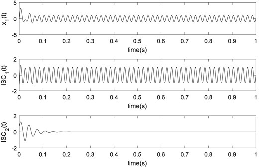
Fig. 4LCD result of x2t=sin⁡100πt+0.5sin⁡50πt+0.5t+1

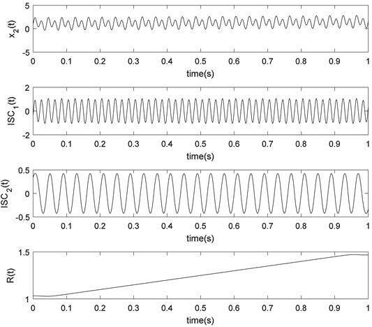
Figs. 3-4 show the LCD results for different signals. Fig. 3 is a graph of $x_1\left(t\right)=\sin \left(100\pi t\right)+3\mathrm{e}\mathrm{x}\mathrm{p}(-10\pi t)\mathrm{s}\mathrm{i}\mathrm{n}\left(60\pi t\right)$ and the ISCs decomposed by using LCD. Fig. 4 is a graph of $x_2\left(t\right)=\sin \left(100\pi t\right)+0.5\sin \left(50\pi t\right)+0.5t+1$, the ISCs and residual decomposed by using LCD.

2.2.3. Comparisons between EMD and LCD

We consider the signal shown in Eq. (18):

18

$x\left(t\right)=x_1\left(t\right)+x_2\left(t\right),$
$x_1\left(t\right)=\left[1+0.5\sin \left(10\pi t\right)\right]\mathrm{c}\mathrm{o}\mathrm{s}\left(100\pi t+30\pi t^2\right),$
$x_2\left(t\right)=4\sin \left(40\pi t\right).$

In order to compare LCD with EMD, we now decompose the signal $x\left(t\right)$ using EMD and LCD, respectively.

The waveforms of the signals are shown in Fig. 5. The sampling frequency is 1000 Hz.

Fig. 5Time waveform of the simulated signal represented by Eq. (18)

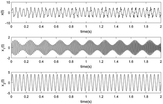
The decomposition results of the simulated vibration signals obtained by EMD and LCD are shown in Figs. 6-7.

Fig. 6EMD results of simulated signals

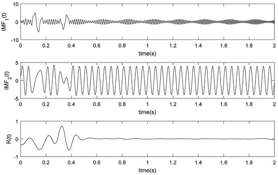
From Figs. 6 and 7 we could find that the two IMFs derived from EMD have the phenomenon of mode mixing, while the LCD method derives a well result matching the true components extremely.

Fig. 7LCD results of simulated signals

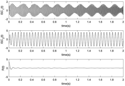
In order to compare them detailed, consuming time and iteration times for getting each IMF and each ISC are considered as evaluation parameters. Besides, since the first two components obtained by EMD and LCD are in accordance with $x_1\left(t\right)$ and $x_2\left(t\right)$, the correlations of the first IMF and ISC with $x_1\left(t\right)$ and the second IMF and ISC with $x_2\left(t\right)$ are considered, respectively. The three evaluation parameters are given in Table 1.

Table 1The comparison parameters of IMF and ISC components

	Time (ms)	Iteration times	Correlation
IMF1	26	8	0.674 5
IMF2	3.6	2	0.958 1
ISC1	1.5	14	0.991 6
ISC2	2	1	0.999 1

From Table 1, it can be found that the consuming time of the two components obtained by EMD are both more than that obtained by LCD. Besides, the correlations of the two ISC components with the true components are higher than that of IMF components’, which means the LCD decomposition results are more close to the true values. Therefore, through this simulation signal, LCD is superior to EMD in certain aspects at least for certain signals.

In EMD, the baseline is defined based on the connection of the whole maxima and minima with cubic spline. The fitting errors generate easily in the boundary for the cubic spline fitting in EMD. In LCD, however, firstly the adjacent maxima (or minima) are connected by straight lines and then the two values at every extrema are averaged respectively. And the baseline is constructed by connecting the obtained values with cubic spline. Hence, in theory LCD has a smaller fitting error and a faster running-time than EMD.

From Eqs. (5)-(6), $g_k$ can be rewritten as:

19

$g_k=a_k{L}_k+a_{k+1}{L}_{k+1}-a_{k+2}{L}_{k+2},$

where:

$a_k=\frac{1}{2}\left[1-\frac{t_{k+1}-t_k}{t_{k+2}-t_k}\right],a_{k+1}=\frac{1}{2},a_{k+2}=\frac{t_{k+1}-t_k}{2\left(t_{k+2}-t_k\right)}.$

In fact, $L_k$ is an ensemble average of three adjacent extrema, meanwhile, the base line is connecting all the $L_k$ with the cubic spline. Hence, LCD has a well local characteristics and a simple geometrical definition, compared with EMD. Therefore, compared with EMD, LCD at least has certain advantages in running time, reducing fitting errors and restraining end effect and mode mixing.

As can be seen from the flowchart, frequency analysis methods based on sparse decomposition, LCD, Hilbert transform and FFT transform are used for the diagnosis of bearing and gear states of the gearbox. We consider the detailed procedure of bearing fault diagnosis.

3. Bearing fault diagnosis algorithm with CS and LCD

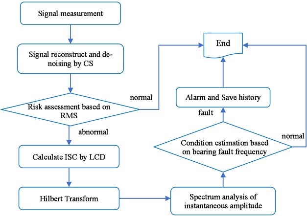
Fig. 8 shows the flowchart of the bearing fault diagnosis algorithm based on CS and LCD.

The calculation and processing procedures of this algorithm are as follows.

Step 1: Measure the vibration from the equipment with the bearing to be tested using a vibration measuring device.

Step 2: Decompose the measured vibration signal into CS and reconstruct it to perform the denoising process.

Step 3: Calculate the RMS value of the denoised vibration signal and calculate the risk determined by the ratio of this value to the allowable vibration RMS value. If the risk is less than the threshold, the bearing is considered normal and finished. If not normal, go to step 4.

Step 4: Decompose the denoised vibration signal obtained in step 2 into LCD to obtain the ISCs.

Step 5: Calculate the instantaneous amplitude by performing a Hilbert transform for the first ISC with lots of fault information.

Step 6: Perform FFT for instantaneous amplitude data.

Step 7: Check whether there is a peak value corresponding to the fault characteristic frequency of the bearing in the power spectrum. If not, it shall be considered normal and finished. If there is a peak value, go to step 8.

Fig. 8The flowchart of the bearing fault diagnosis algorithm

Step 8: Ring the alarm, save the fault history, and finished.

As you can see from the flowchart, we use CS, LCD, Hilbert transform and frequency analysis methods based on FFT transform for the diagnosis of bearing fault. In this section, we consider the detailed procedure of bearing fault diagnosis.

3.1. Reconstruction and de-noising of vibration signals using CS theory

In general, the capacity of the vibration data obtained for a certain period of time is very large. Therefore, data compression methods that can reduce the dimensionality of the collected vibration data while preserving the most useful information are necessary. Sparsity decomposition theory is a new kind of data sampling technique, and using this theory, it is possible to reconstruct the original signal with only a few samples less than the Nyquist sampling rate.

Fig. 9Compression process of vibration signal

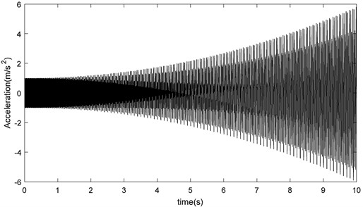
Let us show through the simulation signal that the vibration signal is sparsely represented by the fast Fourier transform matrix. In Fig. 10, the simulated vibration signal, represented by Eq. (20), is shown by a waveform sampled at 1024 Hz:

20

$x\left(t\right)=\cos \left(2\pi \times 80t\right)+0.05t^2\cos \left(2\pi \times 30t+2\right).$

Fig. 10Simulated vibration signal

When performing FFT with 5-5.5 s of data, it can be seen that only a few data points are nonzero, and most of the transform coefficients are zero, as shown in Fig. 11(b).

However, FFT of the noise does not result in zero coefficients at almost all data points. That is, the noise is not sparsely represented by the FFT (Fig. 11(d)).

To validate the de-noising of the vibration signal using CS, the simulated vibration signal, denoted by Eq. (20), was used Fig. 12(a) shows the data of 0-0.1 s in the simulated signal represented by Eq. (20), and the simulated signal added 1dB noise (Fig. 12(b)) to the data is shown in Fig. 12(c). The results of de-noising using compressive sensing are shown in Fig. 13. Fig. 13(a) shows uncontaminated signal and Fig. 13(b) shows contaminated signal (See the Fig. 12(a) and Fig. 12(c)). Fig. 13(c) shows the result of de-noising using CS.

Fig. 11Waveforms of vibration signal and noise and its FFT coefficients

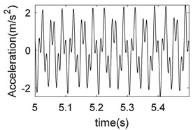
a) The waveform of the vibration signal

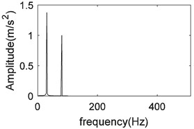
b) FFT coefficients of the vibration signal

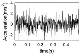
c) The waveform of the noise

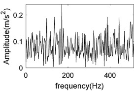
d) FFT coefficients of the noise

Fig. 12Simulated signal

a) Ideal signal

b) Noise

c) Noise-contaminated signal

To quantitatively evaluate the de-noising result, let us calculate the signal-to-noise ratio (SNR) of the de-noising signal. The SN ratio of the de-noising signal can be calculated as follows:

21

$\mathrm{S}\mathrm{N}\mathrm{R}=20\log \left(\frac{{‖x‖}_2}{{‖\widehat{x}-x‖}_2}\right),$

where $\widehat{x}$ is the de-noising signal.

Calculated using Eq. (21), the SN ratio of the de-noising signal was 5.96 dB. It can be seen that the CS theory can reduce the traffic and memory capacity by compressing the signal, and, in addition, the reconstruction process can be further de-noising to extract the signal features more accurately.

Fig. 13Original signal and recovered signal

a) Ideal signal

b) Noisy signal

c) De-noising by CS

Fig. 14Bearing vibration signal

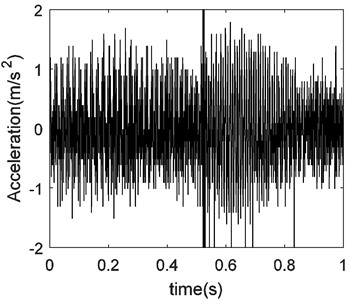
a) The original signal

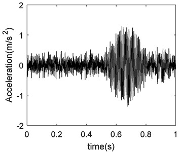
b) The signal recovered by CS

Let us verify the effectiveness of de-noising by compressive sensing theory with field measurement signals. Fig. 14(a) shows the time waveform of bearing vibration signal of the raw material reduction gearbox of the Cement Factory. The de-noising of the signal using the CS theory is shown in Fig. 14(b).

To validate de-noising results, the FFT is shown in Fig. 15. Fig. 15(a) and Fig. 15(b) are FFT of the signal shown in Fig. 14(a) and Fig. 14(b), respectively. As you can see, the CS gives good results for the in field measurement signals.

3.2. Instantaneous amplitude and instantaneous frequency analysis based on LCD and Hilbert transform

When a fault occurs in a rotating machine element such as a gear or rolling bearing, the corresponding vibration signals exhibit amplitude modulation and frequency modulation. To extract the fault feature of the modulated signal, demodulation analysis is widely used, among which the Hilbert transform is one of the most popular demodulation methods because it can effectively extract the envelope of the faulty vibration signal.

Fig. 15Fourier transform result

a) Fourier transform result of the original signal

b) Fourier transform result of the signal recovered by CS

According to the Hilbert transform and analytic signal theory, if for a signal, has relatively low frequency, and has a relatively high frequency, and uncoupled spectrum, then the analytic signal can be expressed in terms of instantaneous amplitude and instantaneous phase as follows:

22

$F\left(t\right)=f\left(t\right)+\mathrm{j}\stackrel{-}{f}\left(t\right)=A\left(t\right)e^{i\phi \left(t\right)}.$

Here, and is the Hilbert transform of:

23

$\stackrel{-}{f}\left(t\right)=\frac{1}{\pi }\underset{-\infty }{\overset{\infty }{\int }}\frac{f\left(\tau \right)}{t-\tau }d\tau .$

The instantaneous frequency is given by the derivative of the time of the instantaneous phase, that is:

24

$f\left(t\right)=\frac{1}{2\pi }\frac{d\phi \left(t\right)}{dt}.$

The condition for and is a kind of narrowband signal condition that the signal must satisfy, and, therefore, according to the analytic signal theory, the envelope and phase of the narrowband signal are the absolute value and phase of the analytic signal, i.e., the instantaneous amplitude and the instantaneous phase.

Generally, the rotary machine fault vibration signal is a multi-component amplitude modulation-frequency modulation signal, which does not satisfy the above conditions.

To solve this problem, a LCD is used to decompose the multi-component signal into single-component ISCs and the fault feature is extracted by applying the Hilbert envelope spectrum to the first few ISCs containing the major fault component.

4. Validation

Bearing vibration data are obtained from Case Western Reserve University [28]. As shown in Fig. 16, the bearing experimental apparatus consists of a 2 hp three-phase motor (left), a torque transducer(middle), a dynamometer (right) and control electronics (not shown). Drive-end bearings of the motor used in the experiments are deep groove ball bearings of type 6205-2RS JEM SKF.

Fig. 16Experimental setup

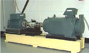
To validate the capability of the proposed method, experimental data analysis on rolling bearing with different categories and severities was conducted. The experimental data are bearing fault data which were derived from the Electrical Engineering Laboratory of Case Western Reserve University (CWRU) [25]. The bearing type is 6205-2RS JEM SKF deep groove ball bearings.

The vibration signals of bearing were collected under four conditions including the normal condition, inner race fault condition (IRF), the outer race fault condition (ORF) (at the 6 o’clock position) and the ball fault condition (BF). The fault bearings are using the electro-discharge machining with fault diameters of 0.1778 mm, 0.3556 mm, 0.5334 mm, and 0.7112 mm to simulate different fault severities. The associated rotating speed of driving motor is set to be 1730, 1750, 1772 and 1797 rpm, respectively. The sampling rate of the data acquisition device is set to 12,000 Hz and the sampling time is 1s. In this work, two different bearing datasets are provided. The details about these two bearing datasets are shown in Table2.

The time domain waveforms of vibration signals under outer race fault are shown in Fig. 17, respectively. In order to account for field conditions, the Gaussian random noise was added.

Fig. 17The time domain waveforms of vibration signals under outer race fault

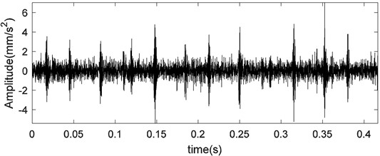
When a fault occurs in a rolling bearing, the vibration signal is usually a multi-component signal containing noise. Thus, first of all, the CS theory is used to remove noise and compress the data, and the LCD is used to decompose the signal into ISCs. The first three ISCs are shown in Fig. 18.

The corresponding Hilbert envelope spectrum obtained by Hilbert transform of the first ISC is shown in Fig. 19. In Fig. 19, we can see spectrum lines at the characteristic frequency of the outer race fault (107.31 Hz) and its harmonic frequency.

Fig. 18LCD result of bearing vibration signal shown in Fig. 17

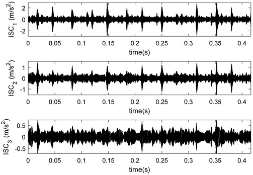
Fig. 19Hilbert envelope spectrum of the first ISC component

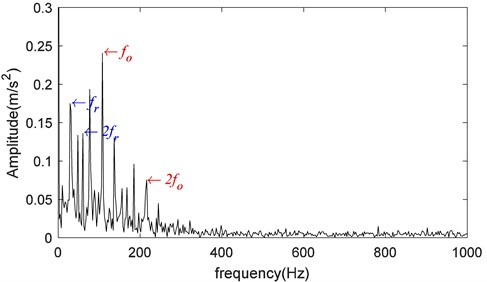
Fig. 20The time domain waveforms of vibration signals under inner race fault

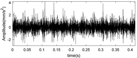
Fig. 21LCD result of bearing vibration signal shown in Fig. 20

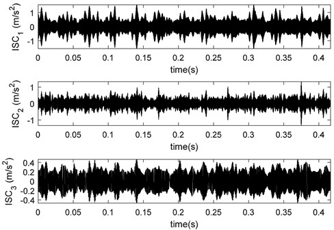
Fig. 22Hilbert envelope spectrum of the first ISC component

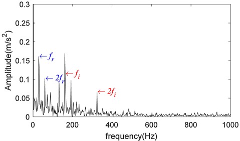
The same procedure was repeated for the bearing vibration signal with the inner race fault. The time domain waveforms of vibration signals under inner race fault and its first three ISCs are shown in Figs. 20-21. And the Hilbert envelope spectrum of the first ISC is shown in Fig. 22. From the spectrum, we can also realize spectrum lines at the characteristic frequency of the inner race fault (162.09 Hz) and its harmonic frequency.

5. Conclusions

In this paper, we proposed a method for detecting rolling bearing faults based on CS theory and LCD and verified its effectiveness. LCD is a new signal processing method, which uses simulated signals to decompose signals, resulting in a 17.9 % higher accuracy compared to the widely used EMD. We also applied CS theory to verify that the fault can be detected by only a few samples without completely reconstructing the vibration signal. Further research on the determination of sparsity $k$ and number of compressed samples $M$ and the computational time reduction of signal processing algorithms for signal reconstruction is needed to improve the efficiency of equipment fault diagnosis using CS theory.