Abstract
The signals emanating from the bearings are complex and contribute to various distributions. The effect of the distribution and mathematical operations are responsible for the change in the statistical moments. This paper investigates the effect of noise on statistical moments of the bearing vibration signals. Initially, the distribution function for Healthy, inner race defect (IRD), outer race defect (ORD), and ball defect (BD) are tested using Kolmogorov Smirnov test (K-S test). The resulting distributions obtained from the K-S test are normal and Laplacian distributed patterns and convey the faulty state of the bearings. The change in noise levels and their influence on the statistical moments are verified. It is observed, the kurtosis for IRD and ORD decreases with increase in noise, whereas, the trend increases for healthy and BD faults.
1. Introduction
Vibration signals analysis is a classical method for detecting bearing faults. The nonlinearity along with the non-stationary property of the bearing signals can alter the probability distribution functions (pdf). The extraction of the signal depends on how closely the basis function matches to the signal. The shape of the pdf clearly demonstrates the true nature of the basis functions. In practical cases, the signal can converge to one or many of the distributions based on the sample length chosen for the observations [1], and it also shows more bias towards sampling rate of the data acquisition device [2, 3]. Kurtosis depends on the shape factor rather than the amplitude of the signal, and shape factor, in turn, depends on the distributions [4]. The analysis of pdf can be carried out using different methods, like Kolmogorov Smirnov test (K-S test), Anderson Darlington test, Chi- Square test, Shapiro-Wilk normality test [5, 6].
Once the signals are decoded to a particular distribution, the fault signal can be extracted easily even if the signals are buried in the noise. Even though it seems to be the solution to many problems, still, the ambiguity in the extraction persists due to ignorance and understanding of the true nature of the mathematical operators the signal built with. The vital part in the signal analysis is the initial study on the behavior and then extracting the information. The fault analyses of bearing using a different flavors of kurtosis have been reported in the literature. The kurtosis can be calculated in the time domain, frequency domain, and time-frequency domain as well [7, 8]. The kurtosis and their distribution function have a significant impact in signal detection [9]. The influence of different mathematical operators can change the statistical properties of the signals [10]. In bearing fault analysis, the Hilbert transform is used as to demodulate the modulated signals [11, 12]. Likewise, the logarithm function is applied to the FFT to separate out the side band components present in the signals and this is referred as cepstrum analysis once the signals are transferred to the time domain using inverse IFFT [13].
2. Methodology
The signals and the experimental test bench from the Case Western Reserve University (http://data-acoustics.com/measurements/bearing-faults/bearing-5/) is used for fault identification of bearing. The setup uses a 2 hp motor, a torque transducer/encoder, a dynamometer and a 6205-2RS deep groove ball bearing as shown in Fig. 1. Two different faults of 0.1778 mm/0.007” and 0.5334 mm/0.021” diameter are created in the inner race, outer race and on the ball using electro-discharge machining (EDM). Drive end vibration data of the bearing are collected using an accelerometers sensor mounted at 6 o’clock positions. The vibration signals are acquired using 16 channel data acquisition card and at a sampling rate of 12000. Table 1 represents the bearing configuration.
Fig. 1Experimental setup for bearing vibration analysis
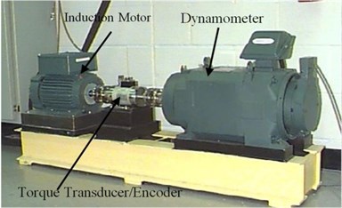
Table 1Ball bearing configuration
Bearing type | Pitch dia. (in) | Rolling element dia. (in) | Number of rolling element |
6205-2RS JEM SKF (DGBB) | 1.537 | 0.3125 | 9 |
3. Results and discussion
The pdf of the vibration signals depends on sampling duration and sampling rate. But, for this study the distribution function are tested for a duration of around 10 sec and sampling rate of 12000. Initially the results are analyzed using K-S test to identify the closest distribution.
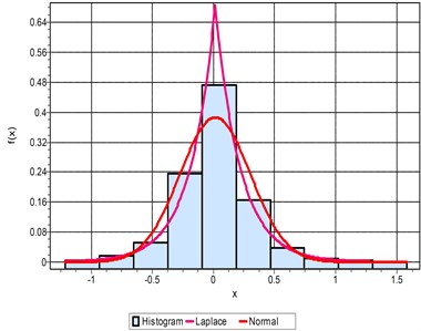
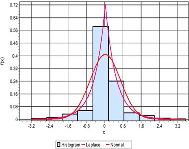
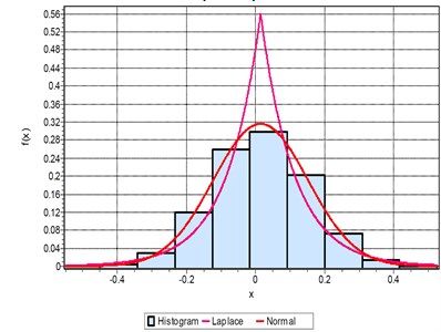
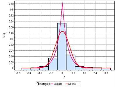
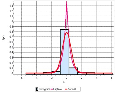
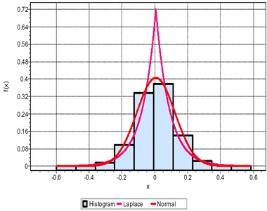
Fig. 3(a) shows the pdf and the histogram for IRD defect. It is observed that the pdf is closer to Laplace distribution with a value of 0.64 and least significant for the normal distribution. The boundary value of x ranges between 1.5 to –1.2. For ORD fault in Fig. 3(b) the pdf increases to 0.72 and the boundary value is, –3.2 < x < 3.3. The analysis also shows that ORD fault distribution is close to Laplace rather normal for a fault dimension of 0.007”. When the K-S test is conducted for BD, the histogram and pdf are closer to the normal distribution as in Fig. 3(c). When the K-S test is used to verify the fault for a higher dimension fault size of 0.021”, the pdf as well as the boundary condition increases to limiting value of –3.2 <x< 3.2 as compared to –1.2 < x < 1.5 as shown in Fig. 3(d). The ORD has the maximum range for the boundary limiting the signal as well as the pdf. The pdf value is more than 1.3 and the boundary range from –6 < x < 6 as compared to –3.2 < x < 3.3 as shown in Fig. 3(e). The signal follows the Laplacian distribution closely rather the normal distributions. The same analysis when applied to the BD, the boundary is limited to a smaller range with pdf of 0.72 as shown in 3(f). It can be concluded that the ORD and IRD faults follow the Laplace distribution and the BD follow the normal distributions Irrespective of the fault sizes. Only the deviation happens to be along the boundary and the value of the pdf. More the fault size the higher the value of pdf as well as boundary values.
As the signal gaussian and Laplacian noise are commonly observed in bearing vibration signals, the authors have tried to analyze the effect of the noise generated using these two distributions on the kurtosis of the signal and best possible method to enhance the kurtosis. In this approach, four different signals are generated by adding Gaussian and Laplacian noises in percentage of the RMS value of the signal. It can be observed from Table 2 that after adding noise to the healthy bearing signals, the kurtosis started rising from 2.802 to 2.915, and it indicates the change in the shape parameter.
Fig. 3Probability density function of: a) IRD, b) ORD, c) BD for 0.007”, d) IRD, e) ORD, f) BD for 0.021” fault dimensions
a)
b)
c)
d)
e)
f)
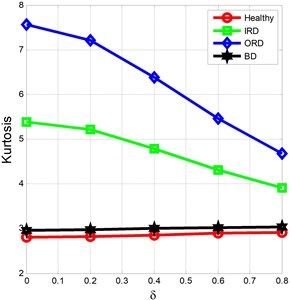
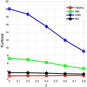
Similar observations are true for the ball defects i.e. the kurtosis increases with increase in noise i.e. from 2.952 to 3.037. But dramatic changes are observed for IRD and ORD. The kurtosis started falling with increased noise intensities. The kurtosis value decreases from 5.380 to 3.910 for IRD, and 7.556 to 4.685 for ORD as shown in Fig. 4(a). It can be inferred that the vibration signature for healthy, BD, IRD and ORD exhibit different distribution as the noise are introduced into the signals. The similar change in the kurtosis values for different δ and for higher fault dimensions is shown in Fig. 4(b). The CF for healthy, ORD, and BD increases with addition of noise where as it decreases for IRD. The other statistical parameters do not show any regular pattern to conclude about noise and their effects.
Table 2Statistical moments for healthy, IRD, ORD and BD (0.007”) for Gaussian noise
p | Mean | RMS | Var | SD | PV | CF | SK | KS | CLF | IF | |
Healthy | 0 | 0.011 | 0.073 | 0.005 | 0.072 | 0.260 | 3.534 | –0.076 | 2.802 | 74.106 | 4.394 |
0.2 | 0.011 | 0.075 | 0.005 | 0.074 | 0.265 | 3.533 | –0.074 | 2.821 | 72.775 | 4.395 | |
0.4 | 0.011 | 0.079 | 0.006 | 0.078 | 0.300 | 3.785 | –0.066 | 2.857 | 73.881 | 4.710 | |
0.6 | 0.011 | 0.085 | 0.007 | 0.085 | 0.339 | 3.949 | –0.058 | 2.891 | 71.230 | 4.916 | |
0.8 | 0.011 | 0.094 | 0.008 | 0.0939 | 0.378 | 4.000 | –0.050 | 2.915 | 66.003 | 4.996 | |
IRD | 0 | 0.014 | 0.289 | 0.083 | 0.289 | 1.398 | 4.832 | 0.130 | 5.380 | 32.44 | 6.735 |
0.2 | 0.014 | 0.294 | 0.0867 | 0.294 | 1.457 | 4.941 | 0.121 | 5.212 | 31.96 | 6.825 | |
0.4 | 0.014 | 0.311 | 0.096 | 0.310 | 1.552 | 4.987 | 0.099 | 4.790 | 29.216 | 6.735 | |
0.6 | 0.014 | 0.337 | 0.113 | 0.336 | 1.670 | 4.954 | 0.073 | 4.312 | 25.617 | 6.541 | |
0.8 | 0.014 | 0.370 | 0.136 | 0.369 | 1.810 | 4.889 | 0.049 | 3.910 | 22.241 | 6.345 | |
ORD | 0 | 0.032 | 0.661 | 0.436 | 0.660 | 3.380 | 5.108 | 0.064 | 7.556 | 20.844 | 8.393 |
0.2 | 0.033 | 0.676 | 0.455 | 0.675 | 3.429 | 5.073 | 0.044 | 7.214 | 18.853 | 8.041 | |
0.4 | 0.034 | 0.715 | 0.510 | 0.714 | 3.600 | 5.034 | 0.023 | 6.384 | 15.524 | 7.476 | |
0.6 | 0.035 | 0.775 | 0.599 | 0.774 | 3.771 | 4.864 | 0.007 | 5.458 | 12.384 | 6.834 | |
0.8 | 0.036 | 0.851 | 0.724 | 0.851 | 3.965 | 4.655 | –0.002 | 4.685 | 9.970 | 6.288 | |
BD | 0 | 0.015 | 0.137 | 0.018 | 0.136 | 0.541 | 3.935 | –0.022 | 2.952 | 44.661 | 4.919 |
0.2 | 0.014 | 0.140 | 0.019 | 0.139 | 0.568 | 4.046 | –0.013 | 2.979 | 45.125 | 5.064 | |
0.4 | 0.014 | 0.148 | 0.0214 | 0.147 | 0.613 | 4.135 | –0.005 | 3.004 | 43.807 | 5.185 | |
0.6 | 0.014 | 0.160 | 0.025 | 0.160 | 0.664 | 4.134 | 0.0007 | 3.023 | 40.475 | 5.188 | |
0.8 | 0.014 | 0.176 | 0.031 | 0.176 | 0.716 | 4.052 | 0.004 | 3.037 | 36.096 | 5.084 | |
Var: Variance, SD: Standard Deviation, PV: Peak Value, CF: Crest Factor, SK: Skewness, KS: Kurtosis, CLF: Clearance Factor, IF: Impulse Factor. | |||||||||||
Table 3Statistical parametric results for healthy, IRD, ORD and BD (0.007”) for Laplacian noise
– | p | Mean | RMS | Var | SD | PV | CF | SK | KS | CLF | IF |
Healthy | 0 | 0.011 | 0.073 | 0.005 | 0.072 | 0.260 | 3.534 | –0.076 | 2.802 | 74.106 | 4.394 |
0.2 | 0.011 | 0.075 | 0.005 | 0.074 | 0.274 | 3.650 | –0.060 | 2.840 | 75.220 | 4.545 | |
0.4 | 0.011 | 0.079 | 0.006 | 0.078 | 0.342 | 4.300 | –0.041 | 2.954 | 84.477 | 5.375 | |
0.6 | 0.011 | 0.086 | 0.007 | 0.085 | 0.415 | 4.826 | –0.024 | 3.166 | 88.638 | 6.071 | |
0.8 | 0.011 | 0.094 | 0.008 | 0.093 | 0.489 | 5.173 | –0.012 | 3.456 | 88.151 | 6.570 | |
IRD | 0 | 0.014 | 0.289 | 0.083 | 0.289 | 1.398 | 4.832 | 0.130 | 5.380 | 32.443 | 6.735 |
0.2 | 0.014 | 0.294 | 0.086 | 0.293 | 1.419 | 4.824 | 0.110 | 5.210 | 31.261 | 6.662 | |
0.4 | 0.014 | 0.310 | 0.095 | 0.309 | 1.562 | 5.037 | 0.083 | 4.822 | 29.930 | 6.838 | |
0.6 | 0.014 | 0.335 | 0.112 | 0.335 | 1.732 | 5.165 | 0.056 | 4.479 | 27.636 | 6.919 | |
0.8 | 0.013 | 0.367 | 0.135 | 0.367 | 2.013 | 5.470 | 0.036 | 4.316 | 26.340 | 7.282 | |
ORD | 0 | 0.032 | 0.661 | 0.436 | 0.660 | 3.380 | 5.108 | 0.064 | 7.556 | 20.844 | 8.393 |
0.2 | 0.031 | 0.673 | 0.453 | 0.673 | 3.301 | 4.898 | 0.055 | 7.170 | 18.312 | 7.775 | |
0.4 | 0.031 | 0.711 | 0.504 | 0.710 | 3.555 | 4.999 | 0.046 | 6.352 | 15.912 | 7.521 | |
0.6 | 0.031 | 0.769 | 0.590 | 0.768 | 3.891 | 5.058 | 0.039 | 5.542 | 13.692 | 7.300 | |
0.8 | 0.031 | 0.844 | 0.712 | 0.843 | 4.347 | 5.147 | 0.036 | 4.984 | 12.037 | 7.234 | |
BD | 0 | 0.015 | 0.137 | 0.018 | 0.136 | 0.541 | 3.935 | –0.022 | 2.952 | 44.661 | 4.919 |
0.2 | 0.015 | 0.140 | 0.019 | 0.139 | 0.543 | 3.876 | –0.020 | 2.969 | 43.220 | 4.847 | |
0.4 | 0.015 | 0.147 | 0.021 | 0.147 | 0.605 | 4.094 | –0.016 | 3.035 | 43.445 | 5.128 | |
0.6 | 0.015 | 0.159 | 0.025 | 0.159 | 0.745 | 4.666 | –0.010 | 3.186 | 46.251 | 5.873 | |
0.8 | 0.015 | 0.175 | 0.030 | 0.174 | 0.892 | 5.090 | –0.003 | 3.412 | 46.702 | 6.455 |
For significant fault identification in buried noisy signals, proper noise reduction algorithm must be chosen to extract the information from the noise. It is reported in the literature by B. Eftekharnejad et al., that the CF can be used as an indicator for SNR (signal to noise ratio) calculations [14]. It is observed from Table 2 that the CF increases for healthy bearing data (3.534 to 4.000) and for BD (3.935 to 4.052) defects, even after the addition of Gaussian noise of variable intensities. But, the intensity crumbles between 4.832 to 5.470 for IRD, and it decreases for ORD (5.108 to 4.655). It can be verified from the results that CF as a calculator for SNR can misjudge the statistical way of analyzing the signals.
To actuate more information, Laplacian noise is added to the signals as shown in Table 3. It is observed the CF for the Healthy, IRD, ORD, BD faults are ranges between 3.534-5.173, 4.832-5.470, 5.108-5.147, and 3.935-5.090 respectively. CF increases for Healthy, IRD, and BD defects, whereas it decreases for ORD. Both the data having different conjecture in analyzing the CF under variable noise added to the signals. It can also be observed that due to the addition of Gaussian and Laplacian noises the skewness of the signals for IRD and ORD defect moves towards zero i.e. from positive to zero. The skewness for BD and healthy signals moves from negative to zero as shown in Tables 2 and 3. It can be inferred from the analysis that the distribution of the signal can be either Gaussian or Laplacian or can be of mixed types (most likely ranking of the distribution are taken into account). The rank wise analysis shows that the BD and Healthy bearing for .007 and .021 defects best fit to the normal distribution. It can be concluded that the increases in kurtosis may not indicate the improvement SNR (signal to noise ratio) as BD and healthy states of the bearings are concerned. The analysis is true only for the IRD and ORD cases.
Fig. 4Impact of noises on kurtosis for Healthy, IRD, ORD, BD: a) 7 mil, b) 21 mil
a)
b)
4. Conclusions
Firstly, this paper verifies the signal type and their distribution using K-S test. Secondly, it analyzes the effect of different concentration of noise on the statistical moments of bearing faults. The K-S test is significant in finding the exact distribution of the bearing signals as the fault dimension increases. The estimated probability density function for the IRD and ORD follow Laplacian distribution. Whereas, healthy and BD follows normal distribution. It is observed the boundary value can be used as an indicator in detecting a fault. It increases with increase in fault dimension and reflects the closeness of particular fault to the sensor mounting positions. Likewise, the magnitude of the pdf also indicates the qualitative increase in the fault dimension. The doping of noise into the signals indicates the decrease in the fourth order moment for IRD and ORD. But it increases for the healthy and the BD. It is also observed the statistical moments of the healthy and BD are much closer with a little deviation in the kurtosis.
References
-
Walck C. Hand-Book on Statistical Distributions for Experimentalists. University of Stockholm, 2007.
-
Rosser G., Fletcher A. G., Maini P. K., Baker R. E. The effect of sampling rate on observed statistics in a correlated random walk. Journal of Royal Society of Interface, Vol. 10, Issue 85, 2013, p. 1-11.
-
Schwede R. L., Cirpka O. A., Nowak W., Neuweiler I. Impact of sampling volume on the probability density function of steady state concentration. Water Resource Research, Vol. 44, 2008, p. W12433.
-
Decarlo L. T. On the meaning and use of kurtosis. Psychological Methods, Vol. 2, Issue 3, 1997, p. 292-307.
-
Broom M., Nouvellet P., Bacon J. P., Waxman D. Parameter-free testing of the shape of a probability distribution, Biosystems, Vol. 90, Issue 2, 2007, p. 509-515.
-
Park H. M. Univariate Analysis and Normality Test Using SAS. Technical reports, 2006.
-
Randall R. B., Antoni J. Rolling element bearing diagnostics – a tutorial. Mechanical Systems and Signal Processing, Vol. 25, Issue 2, 2011, p. 485-520.
-
Kang M., Kim J., Wills L. M., Member S., Kim J. Time-varying and multiresolution envelope analysis and discriminative feature analysis for bearing fault diagnosis. IEEE Transactions on Industrial Electronics, Vol. 62, Issue 12, 2015, p. 7749-7761.
-
Westfall P. H. Kurtosis as peakedness, 1905-2014. R.I.P. Journal of the American Statistical Association, Vol. 68, Issue 3, 2014, p. 191-195.
-
Balakrishnan A. V. Effect of linear and nonlinear signal processing on signal statistics. Radio Science, Vol. 68, Issue 9, 1964, p. 953-965.
-
Klingspor M. Hilbert Transform: Mathematical Theory and Applications to Signal Processing. Master Thesis, Linköping University, 2015.
-
Johansson M. The Hilbert Transform. Master Thesis, Vaaxjao University, 1999.
-
Randall R. B. A history of cepstrum analysis and Its application to mechanical problems. International Conference Surveillence 7, 2013.
-
Eftekharnejad B., Carrasco M. R., Charnley B., Mba D. The application of spectral kurtosis on acoustic emission and vibrations from a defective bearing. Mechanical Systems and Signal Processing, Vol. 25, Issue 1, 2011, p. 266-284.

