Abstract
Aiming at low efficiency of existing sliding bearing load balance calculation, a new method that based on neural network proportional-integral-derivative (PID) algorithm is proposed for the first time, in which a compound control algorithm combining neural network and PID algorithm is applied. In this new method, the load error is taken as the input of the system, and the eccentricity of the bearing is used as the input of the controller, and the output of the system is the oil film force of the bearing. Comparing with traditional method, calculation results show that: the number of iterations calculated by neural network PID algorithm is less than traditional one and has higher efficiency and stronger adaptability under different loads.
1. Introduction
Sliding bearings have a wide range of applications in large machineries [1]. Load balance calculation is the basis for calculation of dynamic characteristics of sliding bearings, whose results will change with different load conditions. The oil film pressure obtained under the given load needs to meet the load balance condition [2], because the oil film bearing capacity is not necessarily equal to the load when the oil film pressure converges.
At present, the researchers have done a lot of research on the sliding bearing [3, 4], which effectively reveals the lubrication characteristics of the bearing and its influencing factors, but there are relatively few research methods for the calculation of bearing load balance. In this paper, the sliding bearing is taken as the research object, and the mathematical model of fluid lubrication is established. The idea of control system is introduced into the calculation of load balance, and the neural network PID algorithm is used to effectively solve the problem of low computational efficiency and poor adaptability of traditional methods, which has certain reference significance for subsequent research.
2. Sliding bearing model
2.1. Oil film pressure solution
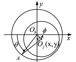
The dynamic pressure radial sliding bearing is simplified, and the oil film thickness calculation is shown in Fig. 1.
In Fig. 1, Ob is the center of the bearing, Oj(x,y) donates the center of the journal. R represents the bearing radius, r is the journal radius, e donates the eccentricity, ϕ is the position angle, and h is the oil film thickness at point A, θ donates shaft rotation angle. According to the geometric relationship, the expression of the oil film thickness is h=C+xcosθ+ysinθ, where C=R-r donates the radius gap, the eccentricity is ε=e/C. The relationship between axial coordinate and the eccentricty position and angle is:
Under certain assumptions, unsteady Reynolds equations [5] can be obtained in an incompressible (invariant), laminar state (without considering turbulence effects) and viscosity does not change with pressure:
where p donates oil film pressure, z donates width of bearing, ω0 represents journal angular velocity, η is oil viscosity. By using the finite difference method and substituting the boundary conditions to solve the Reynolds equation, the pressure distribution of the bearing oil film can be obtained.
Fig. 1Oil film thickness diagram of dynamic pressure sliding bearing

2.2. Bearing oil film joint force solution
Through the known oil film pressure, the resultant oil film force can be integrated, and the oil film joint force is the embodiment of bearing bearing capacity. The oil film pressure is integrated in the x and y directions to obtain the oil film force Fx and Fy:
The discretization of the oil film force is solved, and the double integral is converted into the cumulative summation for calculation. The component in the x direction is P(i,j)cos(θi), and the component in the y direction is P(i,j)sin(θi). Therefore, the oil film force component discretization summation formula is in the form:
where λ is a coefficient whose value is 1/4 of the vertices of the summation region, 1/2 for the boundary, and 1 for the internal node. The oil film resultant force is: F=√ˉF2x+ˉF2y and the load angle is tanφ=ˉFy/ˉFx.
3. Load balance calculation
3.1. Calculation process
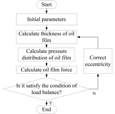
Under the condition of load and other parameters, a set of pressure solutions that reach the convergence condition is calculated by the Reynolds equation iteration, and then the bearing oil film force is solved by integral, and whether the load balance condition is satisfied is judged. If the load balancing condition is not met, the bearing eccentricity needs to be modified until the resulting oil film force satisfies the load balancing condition. The calculation process is shown in Fig. 2.
The load balancing condition is ΔW=|W-F|≤δw, where ΔW is the load error, W donates the external load, and δw is the load balance tolerance. Under certain premise, the size of the oil film force is related to the eccentricity. Therefore, when solving the oil film pressure, it is necessary to find the eccentricity, so that the oil film combined force is equal to the bearing load. The difficulty of the above solution process is how to modify the eccentricity according to the load error, in order that the calculated oil film force can quickly and accurately approach the external load, which requires the algorithm to be simple and efficient, and has strong adaptability.
Fig. 2Flow chart of load balance calculation

3.2. Step-down method
The step-down method is a variable-step load balancing algorithm. The adjustment step size Δε of the fixed eccentricity is not easy to converge, so the general calculation changes the size of the step Δε according to the number of iterations. Primary selection eccentricity ε0, then adjust the eccentricity according to the load error ε:
After k-round calculation, the load error is continuously reduced. At this time, the error value is further reduced by the binary law Δεk=Δεk-1/2 until the convergence accuracy is satisfied. This method is simple, but the problem is how to choose the initial eccentricity ε0 reasonably and how to determine k and start the binary calculation. This method has certain limitations for variable load calculation.
3.3. Single neural network PID method
Neural network PID method has been widely used in control systems [6-8]. The typical single neural network PID control structure is shown in Fig. 3. The characteristic of the algorithm is that the adaptive control function is realized by adjusting the weight coefficients, and the weight coefficient is adjusted according to the supervised Hebb learning rule [9, 10].
Fig. 3Single neural network PID control structure diagram

In order to realize the constraint control of output error and control incremental weighting, with the idea of optimal control, a quadratic performance index is introduced in the adjustment of the weighting coefficient, and the weighting coefficient is adjusted by minimizing the output error and the control incremental weighted square sum. Set performance indicators E(k) as:
where M, N are the weighting coefficients of the output error and the control increment, respectively, and yd(k), y(k) represent the reference input and controller output at time k.
The neuron input u(k) and weight coefficients w(k) are expressed as:
{w'i(k)=wi(k)∑3i=1|wi(k)|,w1(k)=w1(k-1)+ηIK[Pb0z(k)x1(k)-QK∑3i=1(wi(k)xi(k))x1(k)],w2(k)=w2(k-1)+ηPK[Pb0z(k)x2(k)-QK∑3i=1(wi(k)xi(k))x2(k)],w3(k)=w3(k-1)+ηDK[Pb0z(k)x3(k)-QK∑3i=1(wi(k)xi(k))x3(k)],
where ηP, ηI, ηD are the learning rates for adjusting the weighting coefficients of the control parameters P, I, and D respectively, and b0 is the first values of the output response, and there is:
The neural network PID algorithm is applied to the sliding bearing load balance solving problem. The reference input yd in the algorithm corresponds to the bearing load W, the system output y corresponds to the bearing oil film force F, the control quantity u corresponds to the eccentricity ε, and the system control object corresponds to the bearing elastohydrodynamic lubrication. model.
4. Results and discussions
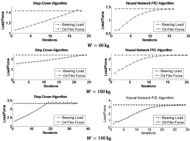
Taking the sliding bearing in Table 1 as the research object, in order to compare the different effects of the step-down method and the neural network PID method under different loads in load balance calculation, the load W is 60 kg, 100 kg and 140 kg respectively. In the calculation process, in order to ensure the gradual reduction of the convergence of the calculation results, the initial value of the eccentricity and the number of iterations before the start of the dichotomy are adjusted. The iterative results are shown in Fig. 4.
Table 1Parameters of sliding bearing
Parameters | Symbol / Unit | Value |
Length | L / m | 0.06 |
Radius | r / mm | 0.045 |
Clearance | C / mm | 2.5×10⁻⁴ |
Oil viscosity | η / Pa·s | 0.015 |
Oil density | ρ / kg/m3 | 876.5 |
Fig. 4Calculation of load balance

It can be seen from the iterative curves in Fig. 4 that these two algorithms can effectively complete the load balance calculation, and as the load increases, the number of iterations increases. Because of the load increasing, it is necessary to increase the eccentricity to produce a large oil film balance, and the greater the eccentricity, the more sensitive the oil film force is to change it. In order to ensure the accuracy of convergence, it is necessary to reduce the eccentricity adjustment step size, thus resulting in an increase in the number of iterations required. When the loads are the same, Fig. 4 indicates that the neural network PID algorithm costs less iterations than the step-down method, and the advantages are more obvious as the load increases.
See Table 2 for specific comparison. When the load is 60 kg, the iterations of the step-down method and the neural network PID method are 18 and 16 times respectively. When the load increases to 100 kg, the number of iterations of the two algorithms is 24 and 20 times. The results demonstrate that neural network PID has strong adaptability. After the system parameters are determined, the calculation step size can be automatically adjusted according to the error.
Table 2Comparison of the numbers of iteration in different algorithms
Load | 60 kg | 100 kg | 140 kg |
Step-down algorithm | 18 | 24 | 34 |
Neural network PID algorithm | 16 | 20 | 19 |
5. Conclusions
In this paper, a new method of load balance calculation of sliding bearing is studied. With the idea of control system, the neural network PID algorithm is applied to the calculation of load balance for the first time. Compared with the traditional step-down method, the neural network can be known from the result. The PID algorithm is obviously superior to the step-down method, and has the characteristics of less iterations, fast convergence, and strong adaptability of working conditions, which can effectively improve the calculation efficiency of the load balance of the sliding bearing.
References
-
Oh K. P., Goenka P. K. The elastohydrodynamic solution of journal bearings under dynamic loading. ASME, Journal of Tribology, Vol. 107, Issue 3, 1985, p. 389-395.
-
Hopf G., Schuler D. Investigation on large turbine bearings working under transitional conditions between laminar and turbulent flow. ASME Journal of Tribology, Vol. 111, 1989, p. 628-635.
-
Tanaka M. Journal bearing performance under starved lubrication. Tribology International, Vol. 33, 2000, p. 259-264.
-
Michaud P., Souchet D., Bonneau D. Thermohydrodynamic lubrication analysis for a dynamically loaded journal bearing. Proceedings of the Institution of Mechanical Engineers, Part J: Journal of Engineering Tribology, Vol. 221, 2007, p. 49-61.
-
Dowon D. A generalized Reynolds equation for fluid-film lubrication. International Journal of Mechanical Science, Vol. 4, 1962, p. 159-170.
-
Chu S. Y., Teng C. C. Tuning of PID controllers based on gain and phase margin specifications using fuzzy neural network. Fuzzy Sets and Systems, Vol. 101, Issue 1, 1999, p. 21-30.
-
Zhang J., Zhang H. Vehicle stability control based on adaptive PID control with single neuron network. International Asia Conference on Information in Control, Automation and Robotics, 2010, p. 434-437.
-
Qi S. F., Wang G. D. PID control of single neuron for switched reluctance motors based on RBF network. Advanced Material Research, Vols. 383-390, 2012, p. 6948-6952.
-
Golea M., Marchand M. Learning curves of the clipped Hebb rule for networks with binary weights. Journal of Physics A General Physics, Vol. 26, Issue 21, 1993, p. 5751.
-
Yin Y., Yuan H., Zhang B. Dynamic behavioral assessment model based on Hebb learning rule. Neural Computing and Applications, Vol. 28, Issue 1, 2017, p. 245-257.

