Contact parameters identification of a cannon cradle and its bushing based on FDA and ELM

Wen, Hao; Hou, Baolin

doi:10.21595/vp.2018.20234

Vibroengineering Procedia

Browse Procedia

Published: 19 October 2018

Check for updates

Contact parameters identification of a cannon cradle and its bushing based on FDA and ELM

Hao Wen¹

Baolin Hou²

^{1, 2}School of Mechanical Engineering, Nanjing University of Science and Technology, Nanjing, China

Corresponding Author:

Baolin Hou

Cite the article Download PDF

Downloads 1246

Abstract

An identification method based on functional data analysis (FDA) and extreme learning machine (ELM) is presented to identify the contact parameters of a cannon cradle and its bushing. A virtual prototype of the cannon is built in ADAMS. The response curves of muzzle vertical acceleration with different contact parameters of the cradle and its bushing are obtained by simulation experiments and used for FDA as sample data. Features of the sample data are extracted by FDA and functional principle component analysis (FPCA), and the features and contact parameters are used to train the ELM. Simulation data and test data are used to verify the proposed method. The presented method is also proved to be feasible and effective by comparing actual muzzle vertical acceleration curve and the muzzle vertical acceleration curve from the virtual prototype with respect to the test data identification results.

1. Introduction

A cradle is the carrier of a cannon recoiling part, which rotates around the trunnion and transfers firing load to other carriages. Changes in contact parameters of the cradle and its bushing will affect mechanism kinematic accuracy during firing and firing accuracy of the cannon. To establish a virtual prototype of the cannon, it is significant to infer the contact parameters of the cradle and the front and back bushing. Due to a cannon is a complex and multi-parameter system, determination of key parameters is a core problem in the modeling process, but these parameters are difficult to measure and can only be obtained by identification.

Since it is difficult to find the analytic expressions of the measurable response to the parameters to be identified, optimization method based on analytic expression cannot be used to identify the contact parameters of the cradle and its bushing [1]. Machine learning (ML) can estimate the dependence of data based on the known sample, so ML can predict and judge the unknown data. Actual experiments can obtain high-quality samples, but for a cannon system, a large number of experiments require a lot of cost and resources and it is easier to obtain samples by virtual simulation.

In this paper, a virtual prototype of the cannon is established, and the response curves of muzzle vertical acceleration are obtained by sampling and simulation experiments of the parameters to be identified and used for FDA as sample data. Using FDA and FPCA to extract the sample data, the extracted features and parameters to be identified are used for ELM training as training samples. Finally, the simulation data and test data are used to identify the parameters and the presented method is proved to be feasible and effective by comparing real muzzle vertical acceleration curve and the muzzle vertical acceleration curve from the virtual prototype with respect to the test data identification results.

2. Modeling and simulation of virtual prototype

The recoiling part of a cannon on zero firing angle is mainly affected by recoil brake force, recuperator force, sealing device friction and cradle rail friction. According to the topological structure of the cannon, the dynamics model is established in ADAMS as shown in Fig. 1.

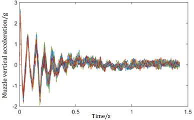
According to the research purpose, the contact parameters to be identified of the cradle and its bushing are the following five parameters: contact stiffness $K_{f}$ and $K_{r}$ , damping $C$ , and clearance $D_{f}$ and $D_{r}$ . Consulting engineering experience, the range of $K_{f}$ is [100000, 200000]N⋅mm, the range of $K_{r}$ is [150000, 300000] N⋅mm, the range of $C$ is [10, 50], and the range of $D_{f}$ and $D_{r}$ is [0.5, 1.5] mm. The five parameters are sampled within the distribution range, and virtual simulation experiments are carried out according to the sampling results. A total of 100 groups of muzzle vertical acceleration curves in counter-recoiling movement are obtained as shown in Fig. 2.

Fig. 1Virtual prototype of the cannon

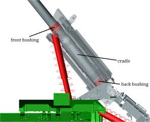
Fig. 2Sample curves of muzzle vertical acceleration

3. Features extraction based on FDA and FPCA

3.1. The FDA and FPCA algorithm

The basic idea of FDA is to treat the observed data as a whole, expressed as a smooth curve or a continuous function, and analyze it from a functional perspective. Assume that the $i$ th observation sample contains a series of observation values $y_{i 1}$ , $y_{i 2}$ , ..., $y_{i n}$ , it can be transformed to be a function $x_{i} (t)$ by FDA, where $t$ is the argument. Generally, the non-periodic data are expanded by the B-spline basis function system. Its functional form is represented by a linear combination of basis functions by letting $c$ indicate the vector of length $K$ and $ϕ$ as the functional vector whose elements are the basis functions $ϕ_{k}$ :

1

x = c^{Τ} ϕ = ϕ^{T} c .

For making the estimated curves more stable, a roughness penalty $P E N_{m} (x)$ is introduced:

2

{P E N}_{m} (x) = \int {[D^{m} x (s)]}^{2} d s = \int {[D^{m} c^{T} ϕ (s)]}^{2} d s = \int c^{T} D^{m} ϕ (s) D^{m} ϕ^{T} (s) c d s = c^{T} R c,

where $D^{m}$ is the m-order derivative and $R = \int D^{m} ϕ (s) D^{m} ϕ^{T} (s) d s$ .

Define $H$ as a weighted matrix and $λ$ as a smoothing parameter, we obtain:

3

{P E N S S E}_{m} (y |c) = (y - Φ c)^{T} H (y - Φ c) + λ c^{T} R c .

The expression for the estimated coefficient vector is:

4

\hat{c} = (Φ^{T} H Φ + λ R)^{- 1} Φ^{T} H y .

FPCA is an expansion of Principle Component Analysis to Hilbert space. According to the derivation of Ramsay [4], the eigenfunction must satisfy the following equation:

5

\int v (s, t) ξ (t) d t = ρ ξ (s),

where $ρ$ is the eigenvalue and $v (s, t) = \frac{1}{N} \sum_{i = 1}^{N} x_{i} (s) x_{i} (t)$ is the covariance function.

Let $ξ$ indicate the eigenfunction and define an integral transform $V$ , $V ξ = \int v (\cdot, t) ξ (t) d t$ , then Eq. (5) can be expressed as:

6

V ξ = ρ ξ .

The principle component function also needs to be smoothed. Maximizing the variance of the samples with a roughness penalty:

7

P C A P S V (ξ) = \frac{v a r \int ξ x_{i} d t}{{‖ξ‖}^{2} + λ \times {P E N}_{2} (ξ)} .

For sample function, the form of basis function combination is $x_{i} (t) = \sum_{k = 1}^{K} c_{i k} ϕ_{k} (t)$ . Let $A$ be the covariance matrix of vectors $c_{i}$ and define $W = \int ϕ ϕ^{T}$ , then Eq. (7) can be written as:

8

P C A P S V = \frac{b^{T} W A W b}{b^{T} W b + λ b^{T} R b} .

The eigenequation corresponding to Eq. (8) is given by:

9

W A W b = ρ (W + λ R) b .

Now, preforming a Choleski factorization $W + λ R = L L^{T}$ and defining $S = L^{- 1}$ , the Eq. (9) can be written as:

10

(S W A W S^{T}) (L^{T} b) = ρ (L^{T} b) .

Defining $u = L^{T} b$ , the Eq. (10) can be written as:

11

(S W A W S^{T}) u = ρ u .

This is a eigenvalue problem, and $u$ , $b$ and the eigenfunction can be carried out in turns.

3.2. Features extraction of muzzle vertical acceleration curves

In this paper, a 4-order B-spline basis function and a 2-order roughness penalty function with smoothing coefficient $λ =$ 50000 are used. Fig. 3(a) shows the sample data for the muzzle vertical acceleration after this functional procedure. Fig. 3(b) shows the first ten principal component functions.

To ensure that the sum of ratio of the principle component functions is greater than 90 %, we select the first 10 principal component functions. For every sample, after it is made to be functional data, the principal component scores can be acquired by calculating the inner product of the functional data and principal component functions, and the principal component scores are the eigenvalues we need.

4. Parameter identification

4.1. ELM algorithm

ELM is a typical single-hidden layer feedforward neural network [9]. Assume any independent sample $(x_{i}, t_{i})$ , $x_{i} = [x_{i 1}, x_{i 2}, . . ., x_{i n}]^{T} \in R^{n}$ , $t_{i} = [t_{i 1}, t_{i 2}, . . ., t_{i m}]^{T} \in R^{m}$ , mathematical model of ELM with $n$ input nodes and $m$ output nodes is:

12

\sum_{i = 1}^{\tilde{N}} β_{i} g_{i} (x_{j}) = \sum_{i = 1}^{\tilde{N}} β_{i} g (w_{i} \cdot x_{j} + b_{i}) = o_{j}, j = 1,2, . . ., N,

where $\tilde{N}$ is the number of hidden layer nodes, $g (x)$ is the activation function, $w_{i}$ is the weight connectiing the $i$ th input node and hidden node, $β_{i}$ is the weight connecting the $i$ th hidden node and output node, and $b_{i}$ is the threshold of the $i$ th hidden node.

Fig. 3The results of FDA and FPCA

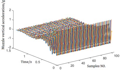
a) Muzzle vertical acceleration after function procedure

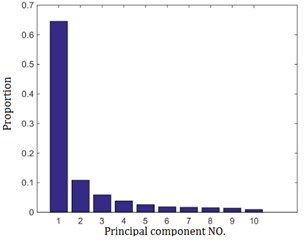
b) Proportion of first ten principal components

When the number of hidden nodes is equal to training samples, ELM can approximate the training sample with zero error. There are $β_{i}$ , $w_{i}$ , $b_{i}$ and output layer matrix $H$ which make:

13

\begin{array}{l} H β = T, \\ H (w_{1}, . . ., w_{\tilde{N}}, b_{1}, . . ., b_{\tilde{N}}, x_{1}, . . ., x_{N}) = {[\begin{matrix} g (w_{1} \cdot x_{1} + b_{1}) & \dots & g (w_{\tilde{N}} \cdot x_{1} + b_{\tilde{N}}) \\ ⋮ & ⋱ & ⋮ \\ g (w_{1} \cdot x_{N} + b_{1}) & \dots & g (w_{\tilde{N}} \cdot x_{N} + b_{\tilde{N}}) \end{matrix}]}_{N \times \tilde{N}} \\ β = {[β_{1} β_{2} . . . β_{\tilde{N}}]}_{\tilde{N} \times m}^{T}, T = {[t_{1} t_{2} . . . t_{N}]}_{N \times m}^{T} . \end{array},

$β$ can be acquired by solving the least squares solution of Eq. (13):

14

\hat{β} = H^{+} T,

where $H^{+}$ is the Moore-Penrose generalized inverse of the output matrix.

The identification accuracy and generalization performance of ELM are evaluated by average relative error $E$ and determination coefficient $R^{2}$ , respectively:

15

E = \frac{|{\hat{y}}_{i} - y_{i}|}{y_{i}}, i = 1,2, . . ., n, R^{2} = \frac{{(l \sum_{i = 1}^{l} {\hat{y}}_{i} y_{i} - \sum_{i = 1}^{l} {\hat{y}}_{i} \sum_{i = 1}^{l} y_{i})}^{2}}{[l \sum_{i = 1}^{l} {\hat{y}}_{i}^{2} - (\sum_{i = 1}^{l} {\hat{y}}_{i})^{2}] [l \sum_{i = 1}^{l} y_{i}^{2} - (\sum_{i = 1}^{l} y_{i})^{2}]} .

4.2. Testing of muzzle vertical acceleration

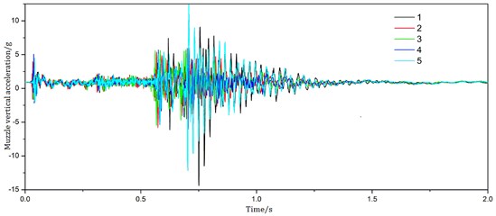
The artificial recoil method is used to test the muzzle vertical acceleration by using the wireless acceleration node A104EX in the wireless test system. Fig. 4 shows the components of the wireless test system. The sensors are installed on the muzzle brake as shown in Fig. 5. The test is repeated 5 times at a firing angle of 0°, and the test results are shown in the Fig. 6.

Fig. 4Hardware components

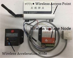
Fig. 5The installation diagram of the sensors

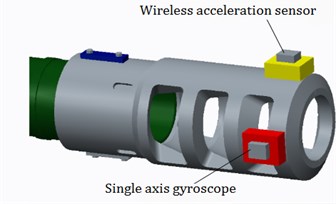
Fig. 6Test curves of muzzle vertical acceleration

4.3. Identification results and analysis

In this paper, 100 groups of sample curves are obtained, of which 95 groups are used for ELM training, and the other 5 groups are used to verify the identification effect of ELM. Table 1 shows the identification results of five contact parameters, and the first five times are the identification results of five groups of simulation data and the last is the identification results of test data. The average relative error $E$ and determination coefficient $R^{2}$ of the identification results are shown in Table 2. The identification results of $E_{f}$ and $E_{b}$ are better and the identification results of $K_{f}$ and $K_{b}$ can also meet the requirements. The identification results of $C$ are relatively poor, and the probable cause is that $C$ has less effect on the muzzle vertical acceleration, or the number of the samples used to train ELM is insufficient.

Table 1Identification results

No. of identification		$C$	$D_{f}$ (mm)	$D_{r}$ (mm)	$K_{f}$ (×10⁵ N⋅mm)	$K_{r}$ (×10⁵ N⋅mm)
1	Real value	21.2857	0.8438	1.2438	1.7786	2.9587
1	Identification value	22.3214	0.8306	1.2275	1.7571	2.9852
2	Real value	17.6429	1.1844	1.1281	1.3293	2.9913
2	Identification value	17.6071	1.1975	1.1206	1.3607	2.8201
3	Real value	24.5357	0.5594	0.9234	1.3929	1.6229
3	Identification value	27.1286	0.5625	0.9313	1.2857	1.9583
4	Real value	21.6929	0.8825	0.6094	1.3536	2.9737
4	Identification value	24.2143	0.9281	0.5813	1.3821	2.8256
5	Real value	27.7143	0.9625	1.0063	1.6393	1.5703
5	Identification value	25.8714	96563	1.0156	1.7071	1.7862
6	Real value	\	\	\	\	\
6	Identification value	14.5357	1.3924	0.8263	2.2214	1.7903

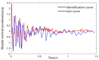
The parameters identified by the test data are substituted into the virtual prototype model for simulation, and the test curve is compared with the simulated curve. As shown in Fig. 7, the two curves are more consistent, which proves the reliability of the identification results.

Table 2Average relative error and determination coefficient

Parameter	Average relative error	Determination coefficient
$C$	8.01 %	0.7681
$D_{f}$	1.40 %	0.9902
$D_{r}$	1.47 %	0.9962
$K_{f}$	3.13 %	0.9035
$K_{r}$	9.12 %	0.9749

Fig. 7Comparison of identification curve and test curve

5. Conclusions

In this paper, a virtual prototype of a cannon is established in ADAMS. The muzzle vertical acceleration curves are obtained by the sampling of the parameters to be identified and simulation experiments and used for FDA as sample data. Using FDA and FPCA to extract the sample data, the extracted features and parameters to be identified are used for ELM training. The simulation data and test data are used to identify the contact parameters of the cradle and bushing. The presented method is proved to be feasible and effective by comparing real muzzle vertical acceleration curve and the muzzle vertical acceleration curve from the virtual prototype with respect to the test data identification results.

References

Zhao Q. Q., Hou B. L. Parameter identification of a shell transfer arm using FDA and optimized ELM. Chinese Journal of Engineering, Vol. 39, 4, p. 611-618.

Search CrossRef
Zong Weiwei, Huang Guang Bin Face recognition based in extreme learning machine. Neurocomputing, Vol. 74, Issue 16, 2011, p. 2541-2551.

Publisher
Ramsay J. O. When the data are functions. Psychometrika, Vol. 47, Issue 4, 1982, p. 379.

Publisher
Ramsay J. O., Hooker G., Graves S. Functional Data Analysis with R and MATLAB. Second Edition, Springer Science + Business Media Inc., New York, 2005.

Search CrossRef
Li M. Analysis of water data function based on principle component analysis method. Natural Sciences Edition, Journal of Hefei University, Vol. 24, Issue 4, 2014, p. 21-25.

Search CrossRef
Zipunnikov V., Caffo B., Yousem D. M., et al. Functional principal component model for high-dimensional brain imaging. NeuroImage, Vol. 58, Issue 4, 2011, p. 772-784.

Publisher
Gao X. X., Sun H. G., Hou B. L., et al. Optimization design of positioning precision for howitzer shell transfer arm with parameter uncertainty. Acta Armamentarii, Vol. 35, Issue 6, 2014, p. 776-781.

Search CrossRef
Huang G. B., Zhao Q. Y., Siew C. K. Extreme learning machine: theory and applications. Neurocomputing, Vol. 70, Issue 1, 2006, p. 489-501.

Publisher

About this article

Received

07 September 2018

Accepted

21 September 2018

Published

19 October 2018

SUBJECTS

Measurements in engineering

DOI

https://doi.org/10.21595/vp.2018.20234

Keywords

parameter identification

functional data analysis

extreme learning machine

cradle

This is an open access article distributed under the Creative Commons Attribution License, which permits unrestricted use, distribution, and reproduction in any medium, provided the original work is properly cited.

Previous article in issue Previous Next article in issue Next

Research article

2023 05 05

Research on fault diagnosis method of electromechanical transmission system based on one-dimensional convolutional neural network with variable learning rate

Liwu Liu, Guoyan Chen, Feifei Yu, Canyi Du, Yongkang Gong, Huijin Yuan, Zhenni Dai

Research article

2021 05 11

Fault recognition of rolling bearing with small-scale dataset based on transfer learning

Ying Wang, Mingxuan Liang, Xiangwei Wu, Lijuan Qian, Li Chen

Research article

2018 10 19

Parameters identification of a cannon counter-recoil mechanism based on PSO and interval analysis theory

Dan Bao, Baolin Hou

Research article

2018 09 24

Rolling bearing fault diagnosis based on EWT and ELM

Shu Xu, Jian Ma

H. Wen and B. Hou, “Contact parameters identification of a cannon cradle and its bushing based on FDA and ELM,” Vibroengineering PROCEDIA, Vol. 20, pp. 202–207, Oct. 2018, https://doi.org/10.21595/vp.2018.20234

Copy Extrica

Copied to clipboard!

TY  - JOUR
DO  - 10.21595/vp.2018.20234
UR  - https://doi.org/10.21595/vp.2018.20234
TI  - Contact parameters identification of a cannon cradle and its bushing based on FDA and ELM
T2  - Vibroengineering PROCEDIA
AU  - Hou, Baolin
AU  - Wen, Hao
PY  - 2018
DA  - 2018/10/19
PB  - JVE International Ltd.
SP  - 202-207
VL  - 20
SN  - 2345-0533
SN  - 2538-8479
ER  - 

Copy Ris

Copied to clipboard!

@article{Hou_2018,
	doi = {10.21595/vp.2018.20234},
	url = {https://doi.org/10.21595/vp.2018.20234},
	year = 2018,
	month = {oct},
	publisher = {{JVE} International Ltd.},
	volume = {20},
	pages = {202--207},
	author = {Baolin Hou and Hao Wen},
	title = {Contact parameters identification of a cannon cradle and its bushing based on {FDA} and {ELM}},
	journal = {Vibroengineering {PROCEDIA}}
}

Copy Bibtex

Copied to clipboard!

[1]B. Hou and H. Wen, “Contact parameters identification of a cannon cradle and its bushing based on FDA and ELM,” Vibroengineering PROCEDIA, vol. 20, pp. 202–207, Oct. 2018, doi: 10.21595/vp.2018.20234.

Copy IEEE

Copied to clipboard!

Hou, Baolin, and Hao Wen. “Contact Parameters Identification of a Cannon Cradle and Its Bushing Based on FDA and ELM.” Vibroengineering PROCEDIA 20 (October 19, 2018): 202–7. https://doi.org/10.21595/vp.2018.20234.

Copy Chicago

Copied to clipboard!

Contact parameters identification of a cannon cradle and its bushing based on FDA and ELM

Abstract

1. Introduction

2. Modeling and simulation of virtual prototype

3. Features extraction based on FDA and FPCA

3.1. The FDA and FPCA algorithm

3.2. Features extraction of muzzle vertical acceleration curves

4. Parameter identification

4.1. ELM algorithm

4.2. Testing of muzzle vertical acceleration

4.3. Identification results and analysis

5. Conclusions

References

About this article

Related Articles