Abstract
Fault diagnosis for bearings is a focus and difficulty in diagnosis research area, so an intelligent diagnosis method using intrinsic time-scale decomposition(ITD) and extreme learning machine (ELM) is proposed in this paper. ITD is a relatively practical non-stationary signal decomposition method, which can decompose non-stationary signal into several components. Then, coefficient of kurtosis was extracted, which was acquired to reduce feature dimensions. Last, in order to reduce man-made interference and increase diagnostic accuracy, ELM was applied to identify and classify bearing states. The experimental result shown that above methods work well in classification and diagnosis for bearings state timely.
1. Introduction
Bearings, which play a key role in rotating machinery, are used to support the system to operate reliably. Bearing accidents lead to trouble of operating machine suddenly, resulting in huge economic consequences [1, 2]. Nevertheless, fault-diagnosis methods make little influence because of the tough and uncontrollable environment [3]. In spite that many fault diagnosis methods have been proposed, few can achieve effective rapid diagnosis, which makes it vital to explore an effective method.
In this paper, intrinsic time-scale decomposition (ITD) method is proposed to realize the multi-scale decomposition of time series signal. For the purpose of obtaining the faulty information efficiently, the decomposed signals are re-processed by extracting its coefficient of kurtosis. In addition, extreme learning machine (ELM) is used to identify and classify the state of bearings effectively and efficiently.
2. Methodology
2.1. ITD algorithm
ITD is a time-frequency analysis algorithm, which can decompose non-stationary signal into intrinsic rotating components and drab trend components [4]. Xt represents the signal to be decomposed, and δ represents a baseline extraction factor which should be defined before the first decomposition. Then, a baseline component and an inherent rotation component can be extracted from the raw signal using δ. The first-decomposition expression of Xt can be described as:
where Lt=δXt represents the baseline component and Ht=(1-δ)Xt represents the inherent rotation component.
ITD method has following advantages:
1) As a kind of local wave decomposition method, the time-frequency resolution is not affected by the time-frequency uncertainty, which means higher temporal resolution and frequency resolution.
2) Compared to the EMD method, ITD needs uncomplicated screening and spline interpolation process, which leads to lower computer processing time.
2.2. ELM algorithm
ELM is a new type of single-hidden-layer feedforward networks (SLFNs) proposed by Huang et al. in 2006 based on the generalized inverse matrix theory. Compared to the traditional neural network, ELM improves the network generalization ability and the learning speed [5, 6]. More specific theories of this method are given in Refs [7-10].
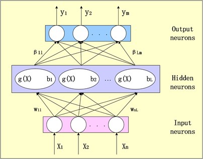
The network structure of ELM is the same as the BP network with single hidden layer, which shows in Fig. 1. About the input layer, xi represents the ith input value and wi=[w1i,w2i,…,wni] represents the vector of input weight which connects the input layer and the hidden layer. About the hidden layer, L represents the total number of hidden neurons, g(x) represents the activation function and bi represents the offset of the ith hidden neuron. About the output layer, βi=[βi1,βi2,…,βim] represents the vector of output weight which connects the hidden layer and the output layer and yj represents the jth output value. The expression of this algorithm can be described as:
Fig. 1The network structure of ELM

2.3. Flow of the proposed method
There are three major steps of the methodology.
Step 1: signal decomposition. ITD decomposes raw signal into finite number of intrinsic rotating component and drab trend component.
Step 2: feature extraction. Coefficients of kurtosis are extracted form decomposed components and the useless coefficients of kurtosis are eliminated.
Step 3: state classification. With the use of coefficient of kurtosis, the state of bearings can be determined by ELM.
3. Experimental verification
3.1. Experiment setup
In this study, the test rig mainly includes one 2000 RPM AC motor, one pulley, one radial load and four bearings. All failures occurred after exceeding designed life time of the bearing which is more than 100 million revolutions. The vibration signals, which includes the normal, inner race fault, outer race fault, were collected by accelerometers installed on bearings with sampling frequency of 20 kHz. There are two sets of data, which include a set of training data and a set of test data. Each set of data include 3 types of bearing state and each state includes 30 sets of data.
3.2. Feature extraction
3.2.1. ITD-based signal decomposition
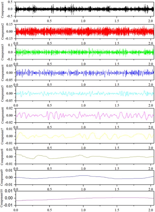
Firstly, ITD was used to decompose non-stationary signal into intrinsic rotating components and drab trend components, which shows in Figs. 2. This step makes it easy to get the fault feature.
Fig. 2ITD decomposition of vibration

3.2.2. Fault feature extraction based on coefficient of kurtosis
The signal obtained by above method, which are a series of decomposing signals, cannot be used to classify directly. To solve this problem, the feature extraction method based on coefficient of kurtosis is required in this study. Coefficient of kurtosis is a dimensionless parameter, which means it has nothing to do with the bearing speed, size and load plus it is sensitive to the vibration signal. Thus, coefficient of kurtosis is applied to reduce feature dimension.
The fault feature values obtained by ITD and coefficient of kurtosis are partly shown in Table 1. The feature information is composed by seven feature values after the removing of useless feature value.
3.3. ELM-based state classification
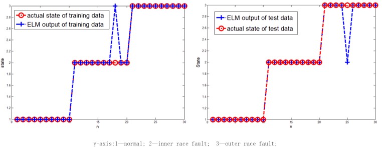
Based on the fault feature extraction methods mentioned, state classification for bearings can be proceeded using ELM. The show results in Fig. 3 which obtained by ELM are good-effective. The left figure as fellow is the classification results of training data while the right figure is the classification result of test data, with both reach the accuracy of 95 % or more.
Table 1Processing result based on ITD and coefficient of kurtosis
State | Fault feature values | ||||||
1 | 2 | 3 | 4 | 5 | 6 | 7 | |
Normal | 5.2489 | 2.4123 | 3.6672 | 3.9192 | 3.7598 | 3.8047 | 2.4836 |
5.4325 | 2.4121 | 3.7764 | 4.7186 | 3.6769 | 3.2378 | 3.4722 | |
5.3731 | 2.3534 | 3.7510 | 4.5026 | 4.3663 | 3.0383 | 2.5094 | |
5.3035 | 2.4303 | 3.6627 | 3.6806 | 3.4660 | 3.1984 | 3.5150 | |
5.6215 | 2.3982 | 3.6608 | 4.2447 | 4.3051 | 3.6260 | 3.0087 | |
Inner race fault | 2.7792 | 3.5932 | 3.1817 | 3.3381 | 3.5932 | 2.8444 | 4.2310 |
2.9310 | 3.4284 | 3.2967 | 3.5655 | 3.9568 | 3.1091 | 2.2796 | |
2.9118 | 3.5717 | 3.2863 | 3.4483 | 3.3746 | 2.8262 | 2.3381 | |
2.8465 | 3.5669 | 3.1945 | 3.1932 | 3.4527 | 3.1717 | 2.5534 | |
2.7734 | 3.4385 | 3.2889 | 3.3134 | 2.9707 | 3.1238 | 2.2935 | |
Outer element fault | 3.6021 | 2.9423 | 3.3990 | 4.3574 | 4.1333 | 4.0896 | 2.8101 |
3.6715 | 3.1132 | 3.4834 | 4.6444 | 3.0684 | 3.6411 | 2.5670 | |
3.8466 | 2.9663 | 3.5001 | 3.3135 | 3.4636 | 4.0476 | 3.4538 | |
4.8541 | 3.0087 | 3.7781 | 3.8116 | 3.9932 | 3.6156 | 2.6074 | |
3.6585 | 2.8554 | 3.5767 | 3.5362 | 3.7804 | 3.2679 | 2.3083 | |
Fig. 3ELM classification effect comparison

4. Conclusions
In this paper, a method for fault diagnosis to bearings using ITD, coefficient of kurtosis and ELM is proposed. The experimental results show that ITD and coefficient of kurtosis work well in signal decomposition and feature extraction while ELM works well in state classification. Thus, the mentioned fault diagnosis method of bearings is reliable and effective.
References
-
Peng Z., Tse P. W., Chu F. A comparison study of improved Hilbert-Huang transform and wavelet transform: application to fault diagnosis for rolling bearing. Mechanical Systems and Signal Processing, Vol. 19, Issue 5, 2005, p. 974-988.
-
Wang Z., Lu C., Wang Z., Ma J. Health assessment of rotary machinery based on integrated feature selection and Gaussian mixed model. Journal of Vibroengineering. Vol. 16, Issue 4, 2014, p. 1753-1762.
-
Tian Y., Ma J., Lu C. Rolling bearing fault diagnosis under variable conditions using LMD-SVD and extreme learning machine. Mechanism and Machine Theory, Vol. 90, 2015, p. 175-186.
-
Sun J., Lu C., Ding Y. Fault diagnosis for hydraulic pump based on intrinsic time-scale decomposition and SoftMax regression. Vibroengineering Procedia, Vol. 10, 2016, p. 229-234.
-
Huang G.-B., Zhu Siew Q.-Y.-C.-K. Extreme learning machine: a new learning scheme of feedforward neural networks. Proceedings of IEEE International Joint Conference on Neural Networks, 2004.
-
Huang G.-B., Zhu Siew Q.-Y.-C.-K. Extreme learning machine: theory and applications. Neurocomputing, Vol. 70, Issue 1, 2006, p. 489-501.
-
Huang G.-B., Ding X., Zhou H. Optimization method based extreme learning machine for classification. Neurocomputing, Vol. 74, Issue 1, 2010, p. 155-163.
-
Huang G.-B., Zhou H., Ding X., Zhang R. Extreme learning machine for regression and multiclass classification. IEEE Transactions on Systems, Man, and Cybernetics, Part B, Vol. 42, Issue 2, 2012, p. 513-529.
-
Huang G.-B. An insight into extreme learning machines: random neurons, random features and kernels. Cognitive Computation, Vol. 6, Issue 3, 2014, p. 376-390.
-
Malathi V., Marimuthu N. S., Baskar S., Ramar K. Application of extreme learning machine for series compensated transmission line protection. Engineering Applications of Artificial Intelligence, Vol. 24, Issue 5, 2011, p. 880-887.
About this article
This study is supported by the Fundamental Research Funds for the Central Universities (Grant No. YWF-17-BJ-J-42 and YWF-16-BJ-J-18) and the National Natural Science Foundation of China (Grant Nos. 51605014 and 51575021), as well as the Technology Foundation Program of National Defense (Grant No. Z132013B002).
