Fault detection in different types of noise environments

Zak, Grzegorz

doi:10.21595/vp.2017.19052

Vibroengineering Procedia

Browse Procedia

Published: 26 September 2017

Check for updates

Fault detection in different types of noise environments

Grzegorz Zak¹

¹Diagnostics and Vibro-Acoustics Science Laboratory, Wrocław University of Science and Technology, Na Grobli 15, 50-421, Wrocław, Poland

Cite the article Download PDF

Downloads 1349

Abstract

Local damage detection is one of the most investigated problems in the field of condition monitoring. Raw signals often possess different components that make it difficult for one to directly detect damage. By such components one can mean high energy of the noise, deterministic part or even artifacts (singular impulses that are not connected to the fault). In this paper author covers problem of the fault detection in different noise environments by means of statistical analysis. Author has applied $α$ -stable distribution as a tool for the impulsivity detection instead of commonly used spectral kurtosis and fractional lower-order covariance as a mean of cyclicity and impulsivity detection in the presence of non-Gaussian noise.

1. Introduction

Local damage detection is currently undergoing major development in terms of the introduced methods and algorithms. In the past years, one can see that this field is growing. Main reason behind interest in this topic is that early local damage detection can prevent further degradation of the elements. Thus, it can reduce costs of operation of whole machine park. One can see works on the machine maintenance in the field [1], application of the data mining methods [2, 3], cyclicity detection [4], signal segmentation via statistical approach [5]. Increasing knowledge of the topic provides us with the ways to extend and merge methods that were often omitted for this field. One of the important problems that is currently investigated in this field is influence and type of the noise that is present in the signal. In case of noise that is non-Gaussian standard methods are not sufficient and one needs to provide another way of analysis. These methods were previously applied to electricity market [6], financial data [7], plasma turbulence [8]. In this paper, author is presenting basic summary of $α$ -stable based methods for the fault detection in different noise environments. Due to the varying behavior of the noise one can divide this problem into three sub-problems. It is known that signal consisting information about the fault will include at least three components:

1) component responsible for the impulsive behavior related to the fault,

2) deterministic component related to the kinematics of the machine,

3) background noise.

One can differentiate at least three types of the background noise. First type, Gaussian, is easiest to proceed with in case of the analysis and signal processing. It does not highly affect most of the algorithms. Second type, Gaussian noise mixed with singular impulses, let us call them artifacts. These impulses are usually connected with the error during signal acquisition, for instance hit on the casing during the measurement. It can affect simple methods used for the informative frequency band selection like spectral kurtosis or kurtogram. Last type of the noise is hardest to work with. It is an impulsive, non-periodic component. It has high energy, usually spread in the whole frequency band. It will highly affect standard methods, mostly rendering them useless. However, there is one more type of the noise. It is a cyclic, impulsive behavior related to the normal work of the machine (see engines, compressors) but it is not a subject of investigation in this paper. The rest of the paper is organized as follows: Section 2 covers main properties of the $α$ -stable distribution and fractional lower-order covariance. In Section 3 author presents application of the methods towards the real world signals. Last section concludes the paper.

2. Methodology

This section covers theory applied to the vibration signals acquired in the harsh environment. Each of these methods is easily applied and consistent with the earlier proposed models of the signal according to the type of the noise. Methods are applied to the time-frequency decomposed signals. As a method of decomposition author used Short-Time Fourier Transform (STFT) and its representation, namely spectrogram. Author reminds the reader; the spectrogram is a square of absolute value of the Short-Time Fourier transform defined for time point $t$ and frequency $f$ as follows [9]:

S T F T (t, f) = \sum_{k = 0}^{n - 1} ‍ x_{k} w (t - k) e^{2 j π f k / N},

where $w (t - τ)$ is the shifted window and $x_{0}, . . ., x_{n - 1}$ is the input signal. Next, let us define $S (t, f) = | S T F T (t, f) |$ .

2.1. The $α$ -stable distribution

In this subsection author introduces the $α$ -stable distribution and present main properties of $α$ -stable distributed random variables. There are few equivalent definitions of $α$ -stable distributed random variables. One of the definition is in terms of its characteristic function.

Namely, a random variable $X$ is said to have $α$ -stable distribution if there are parameters $0 < α \leq 2$ , $σ > 0$ , $- 1 \leq β \leq 1$ and $μ \in R$ such that the characteristic function of $X$ has the following form [10]:

1

ϕ_{X} (t) = E e x p (i t X) = \{\begin{array}{l} e x p \{- σ^{α} | t |^{α} (1 - i β s i g n (t) t a n (\frac{π α}{2})) + i μ t\}, & α \neq 1, \\ e x p \{- σ | t | (1 + i β \frac{2}{π} s i g n (t) l n (| t |)) + i μ t\}, & α = 1 . \end{array}

Properties of the distribution differ according to the change of the parameters. For instance, if the $α$ is lower the data become significantly more impulsive. Interesting property is that with $α < 2$ we do not have finite variance and with $α \leq 1$ we also do not have finite mean. Furthermore, for $β = 0$ we have symmetric distribution, while for positive and negative $β$ we have right-skewed and left-skewed distribution respectively. Parameters $σ$ and $μ$ are stable distribution counterparts of standard deviation and mean.

2.1.1. $α$ -based filter

One of the applications of the $α$ -stable distribution is estimation of the filter characteristic. Since impulsive behavior is one of the indicators of the fault, we can use stability parameter of the mentioned distribution to create a filter characteristic. It is done via estimation of the $α$ for each sub-signal from the time-frequency matrix for the appropriate frequency bin. We define filter characteristic as:

2

α (f) = \frac{m a x_{f} (α) - α (f)}{m a x_{f} (α) - m i n_{f} (α)} .

2.1.2. Fractional lower-order covariance

In case of the impulsive, heavy-tailed noise standard methods are not usually appropriate to deal with it. Impulsive noise can corrupt results since most of the algorithms depends on the impulsivity of the component related to the fault. In such cases it is needed to apply method that connects both impulsivity and cyclicity. It can be achieved using only cyclicity, for instance using Cyclic Spectral Coherence or Cyclic Spectral Density. However, one of the minor disadvantages of these methods is that they rely on the assumption that second moment of the signal is finite. It is often not true in the case of the impulsive behavior present in the data. Thus, there was introduced another measure of the dependency, namely fractional lower-order covariance. It is an appropriate counterpart of the standard dependency measures since it is well-suited for the $α$ -stable distributions (its parameters depend on the stable distribution parameters). Its estimator is easy to apply and has low computational complexity. We define fractional lower-order covariance for the stochastic process $X (t)$ as [11]:

3

R_{x x} (k) = E [X (t)^{< A >} X (t - k)^{< B >}], 0 \leq A, B \leq α / 2,

where $α$ is stability parameter of the fitted $α$ -stable distribution. The estimator of $R_{x x}$ for the set of discrete observations $x_{1}, x_{2}, . . ., x_{N}$ is defined as:

4

R_{x x} (k) = \frac{\sum_{n = L_{1} + 1}^{L_{2}} ‍ | x (n) |^{A} | x (n + k) |^{B} s g n [x (n) x (n + k)]}{L_{2} - L_{1}},

where $L_{2}$ is $m i n (N, N - k)$ , $N$ is equal to signal length, $L_{1}$ is $m a x (0, - k)$ , $0 \leq A$ , $B < α / 2$ and $α$ is estimated stability parameter from the $α$ -stable distribution. Furthemore $< \cdot >$ denotes following operation:

5

z^{< a >} = | z |^{a} s g n z .

Fractional lower-order covariance as a generalized dependency measure can be reduced to the both covariation (particular case of this measure) or to the covariance. It can be done by appropriate choice of the parameters A and B. If sample distribution is Gaussian, then stability parameter is equal to 2. Setting both parameters (A, B) to be equal to their maximum limit ( $α / 2 = 1$ ) results in FLOC measure reducing to the standard covariance.

Algorithm used in this paper applies this measure to the sub-signals extracted from the spectrogram, similary as for the $α$ -stable filter. Further enhancement is done via searching local maxima in the time-lag representation of the FLOC map. Integration of this map allows for the detection of the fault.

3. Results

This section covers application of the methods described in the previous section towards real world signals. There are three cases. First case – vibration signal from the bearing. Background noise is Gaussian. Second case is a vibration signal from the gearbox with artifact (hit on the casing of the gearbox during data acquisition). Last case is a vibration signal from the copper ore crusher with the impulsive noise.

3.1. Case 1 - Gaussian noise

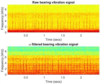
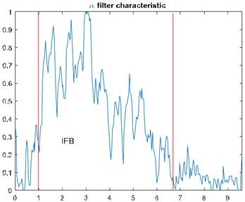
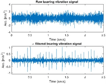
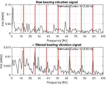
Signal in this case was acquired with frequency sampling equal to 19.2 kHz and signal duration equal to 2.5 s. In this case one will apply $α$ -filter which enhances impulsive behavior related to the fault. $α$ parameter would be lower for the bands with the impulsive behavior. Using simple transformation allows us to obtain filter characteristic which will enhance data in the informative frequency band. In Fig. 1(a) one can see spectrogram of the signal before enhancement (top panel) and its filtered counterpart. It can be seen that noise in the higher frequency band has been attenuated, while impulsive behavior slightly enhanced. In Fig. 1(b) we present filter characteristic for the signal. Fig. 1(c) contains time waveforms before and after filtration. It can be seen that filtration heavily enhanced impulses. In Fig. 1(d) we see that fault frequency 12.69 Hz and its harmonics are easy to notice after filtration.

Fig. 1a) Spectrogram of the raw (top panel) and filtered (bottom panel) signal, b) filter characteristic, c) time waveform of the raw (top panel) and filtered (bottom panel) signal, d) its envelope spectra

a) Spectrogram of the raw (top panel) and filtered (bottom panel) signal, b) filter characteristic, c) time waveform of the raw (top panel) and filtered (bottom panel) signal, d) its envelope spectra

a)

b)

c)

3.2. Case B – Gaussian noise with artifact

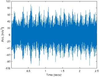
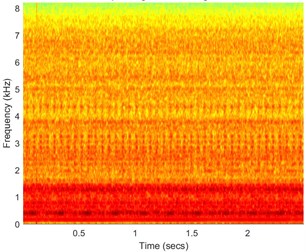
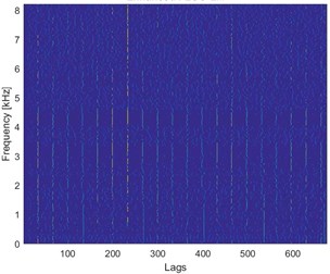
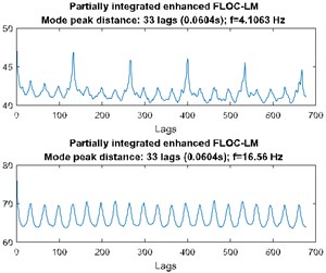
Case B uses FLOC dependency map for the detection of the fault. Most of the standard methods (kurtogram, spectral kurtosis) would produce false results due to the high value of the kurtosis for high frequency bands where one impulses affect whole statistic. Signal was acquired with frequency sampling equal to 16.384 kHz and duration 2.5 s. It can be seen that time waveform (see Fig. 2(a)) has visible impulses repeating around 4 times per second with high amplitude modulation. Decomposing signal to time-frequency representation allows us to see artifact around 0.2 s in band above 7 kHz. Furthermore, cyclic impulsive behavior is visible in band 1.8-5 kHz. Thus, it is reasonable to apply FLOC dependency map and enhance it with local maxima [12]. Result is seen in Fig. 2(c). We can see two types of impulsive behavior. First type with often repetitions in band 1.8-5 kHz and second, previously masked by high energy in band 0.2-1.6 kHz. Partial integration of this map allows to detect both of them with frequencies 16.56 Hz and 4.1063 Hz respectively.

3.3. Case C - heavy-tailed noise

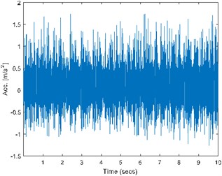
Last type of the analyzed signals has impulsive noise and thus most of the methods cannot be applied due to their high sensitivity towards impulsiveness. Thus, author applied FLOC method that incorporates both impulsiveness and cyclicity. Signal is acquired with 25 kHz frequency sampling and 10 s duration. In Fig. 3(a) one can time waveform of the signal.

Fig. 2a) Time waveform of the signal, b) its spectrogram, c) enhanced FLOC-LM map and d) partially integrated maps

a)

b)

c)

d)

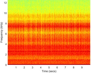
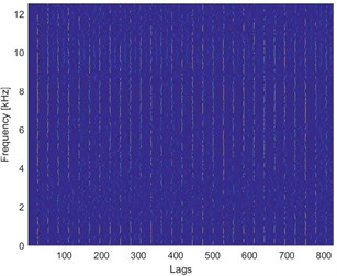
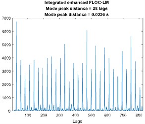
Fig. 3a) Time waveform of the signal, b) its spectrogram, c) enhanced FLOC-LM map and d) partially integrated maps

a)

b)

c)

d)

It can be seen that impulses from the fault and from the ore hitting the inner walls of the ore crusher are not distinguishable. Similarly, one cannot differentiate between them on the spectrogram (see Fig. 3(b)). Applying FLOC method and further, enhancing it by using local maxima method we can see that lag-frequency representation that has evenly spaced impulsive behavior. Integration of this enhanced map and calculation of the distance between peaks (similarly as in the autocorrelation) allows for the fault detection with the frequency of 30 Hz.

4. Conclusions

In this paper, the problem of local damage in different types of noise environments is discussed. Real world signals that are analyzed are often contaminated by noise with varying level of impulsive behavior. Most simple in the signal processing is Gaussian noise. However, it can be seen that this is not common type. Usually, we have artifacts in the signal due to the human error or impulsive behavior due to the type of the machines. The main point of our methodology is to supply the readers with possibility of applying these methods depending on their task. In general, $α$ -filtering is useful substitute of spectral kurtosis due to its insensitivity towards singular impulses (artifacts), while fractional lower-order covariance is a theory-practice consistent method for cyclic impulsive behavior detection.

References

Mcfadden P., Smith J. Vibration monitoring of rolling element bearings by the high frequency resonance technique – a review. Tribology International, Vol. 17, Issue 1, 1984, p. 3-10.

Publisher
Ma X., Nikias C. L. Joint estimation of time delay and frequency delay in impulsive noise using fractional lower order statistics. IEEE Transactions on Signal Processing, Vol. 44, Issue 11, 1996, p. 2669-2687.

Publisher
Samorodnitsky G., Taqqu M. Stable Non-Gaussian Random Processes. Chapman and Hall, New York, 1994.

Search CrossRef
Kruczek P., Obuchowski J., Wylomanska A., Zimroz R. Cyclic sources extraction from complex multiple-component vibration signal via periodically time varying filter. Applied Acoustics, Vol. 126, 2017, p. 170-181.

Publisher
Obuchowski J., Wyłomanska A., Zimroz R. The local maxima method for enhancement of time-frequency map and its application to local damage detection in rotating machines. Mechanical Systems and Signal Processing, Vol. 46, Issue 2, 2014, p. 389-405.

Publisher
Wyłoma´nska A., Zimroz R. Signal segmentation for operational regimes detection of heavy duty mining mobile machines-a statistical approach. Diagnostyka, Vol. 15, Issue 2, 2014, p. 33-42.

Search CrossRef
Wodecki J., Stefaniak P. K., Obuchowski J., Wylomanska A., Zimroz R. “Combination of principal component analysis and time frequency representations of multichannel vibration data for gearbox fault detection. Journal of Vibroengineering, Vol. 18, Issue 4, 2016, p. 2167-2175.

Publisher
Stefaniak P. K., Zimroz R., Bartelmus W., Hardygóra M. Computerised decision-making support system based on data fusion for machinery system’s management and maintenance. Applied Mechanics and Materials, Vol. 683, 2014, p. 108-113.

Publisher
Kruczek P., Wylomanska A., Teuerle M., Gajda J. The modified yule-walker method for a-stable time series models. Physica A: Statistical Mechanics and its Applications, Vol. 469, 2017, p. 588-603.

Publisher
Wyłomanska A., Chechkin A., Sokolov M., Gajda J. Codifference as a practical tool to measure interdependence. Physica A, Vol. 421, 2015, p. 412-429.

Publisher
Wodecki J., Zdunek R., Wyłomanska A., Zimroz R. Local fault detection of rolling element bearing components by spectrogram clustering with semi-binary NMF. Diagnostyka, Vol. 18, Issue 1, 2017, p. 1641-6414.

Search CrossRef
Gajda J., Wyłomanska A. Tempered stable Lévy motion driven by stable subordinator. Physica A: Statistical Mechanics and its Applications, Vol. 392, Issue 15, 2013, p. 3168-3176.

Publisher

About this article

Received

04 September 2017

Accepted

05 September 2017

Published

26 September 2017

SUBJECTS

Fault diagnosis based on vibration signal analysis

DOI

https://doi.org/10.21595/vp.2017.19052

Keywords

α-stable distribution

time-frequency decomposition

local damage detection

Acknowledgements

The work of G. Żak is supported by Statutory Grant No. 0402/0008/17 (G. Żak).

This is an open access article distributed under the Creative Commons Attribution License, which permits unrestricted use, distribution, and reproduction in any medium, provided the original work is properly cited.

Previous article in issue Previous Next article in issue Next

Research article

2018 09 24

Informative frequency band identification method using bi-frequency map clustering for fault detection in rotating machines

Jacek Wodecki, Piotr Kruczek, Justyna Hebda-Sobkowicz, Agnieszka Wylomanska, Radoslaw Zimroz, Konstantinos Gryllias

Research article

2017 03 31

Fault diagnosis of rotating machinery based on time-frequency decomposition and envelope spectrum analysis

Yonggen Chang, Fan Jiang, Zhencai Zhu, Wei Li

Research article

2016 08 31

Generalized dependency maps based on fractional lower order covariance in application to local damage detection

Grzegorz Żak, Agnieszka Wyłomańska, Radosław Zimroz

Research article

2016 06 30

Combination of principal component analysis and time-frequency representations of multichannel vibration data for gearbox fault detection

Jacek Wodecki, Pawel Stefaniak, Jakub Obuchowski, Agnieszka Wylomanska, Radoslaw Zimroz

G. Zak, “Fault detection in different types of noise environments,” Vibroengineering PROCEDIA, Vol. 13, pp. 79–84, Sep. 2017, https://doi.org/10.21595/vp.2017.19052

Copy Extrica

Copied to clipboard!

TY  - JOUR
DO  - 10.21595/vp.2017.19052
UR  - https://doi.org/10.21595/vp.2017.19052
TI  - Fault detection in different types of noise environments
T2  - Vibroengineering PROCEDIA
AU  - Zak, Grzegorz
PY  - 2017
DA  - 2017/09/26
PB  - JVE International Ltd.
SP  - 79-84
VL  - 13
SN  - 2345-0533
ER  - 

Copy Ris

Copied to clipboard!

@article{Zak_2017,
	doi = {10.21595/vp.2017.19052},
	url = {https://doi.org/10.21595/vp.2017.19052},
	year = 2017,
	month = {sep},
	publisher = {{JVE} International Ltd.},
	volume = {13},
	pages = {79--84},
	author = {Grzegorz Zak},
	title = {Fault detection in different types of noise environments},
	journal = {Vibroengineering {PROCEDIA}}
}

Copy Bibtex

Copied to clipboard!

[1]G. Zak, “Fault detection in different types of noise environments,” Vibroengineering PROCEDIA, vol. 13, pp. 79–84, Sep. 2017, doi: 10.21595/vp.2017.19052.

Copy IEEE

Copied to clipboard!

Zak, Grzegorz. “Fault Detection in Different Types of Noise Environments.” Vibroengineering PROCEDIA 13 (September 26, 2017): 79–84. https://doi.org/10.21595/vp.2017.19052.

Copy Chicago

Copied to clipboard!

Fault detection in different types of noise environments

Abstract

1. Introduction

2. Methodology

2.1. The α-stable distribution

2.1.1. α-based filter

2.1.2. Fractional lower-order covariance

3. Results

3.1. Case 1 - Gaussian noise

3.2. Case B – Gaussian noise with artifact

3.3. Case C - heavy-tailed noise

4. Conclusions

References

About this article

Related Articles

2.1. The $α$ -stable distribution

2.1.1. $α$ -based filter