Railway axle box bearing fault identification using LCD-MPE and ELM-AdaBoost

1. Introduction

As a crucial mechanical component, rolling bearings are widely used in subway and railway locomotives [1]. Rolling bearings working status directly affects the operational safety of trains. Thus, the out-of-state identification for axle box bearings is paramount for the detection of hidden dangers, reducing the probability of accidents, ensuring the safety of rail transit, and reliable operation. When a bearing damage or failure occurs, the bearings vibration signals often show non-stationary, non-linear characteristics. Common time-frequency analysis techniques include WVD, STFT, WT, etc., but each one of these methods has its own limitations. For example, the WVD would cause crossing-term interference when dealing with non-stationary signals; the analysis window of STFT needs to be further optimized; the WT has been commonly applied in health monitoring but different mother wavelets should be predefined for each different component. These drawbacks make these classical ways not fully adaptive in nature. The EMD is a self-adaptive time-frequency analysis method. Since the EMD is capable of dealing with non-stationary and non-linear signals, a considerable attention has been attracted to this method in the field of bearing condition monitoring. But the EMD also has a drawback named as the modal mixing nature, and it can cause the distortion of the decomposed IMF [2]. The (LCD) method in the time-frequency analysis is an adaptive, non-stationary signal processing algorithm based on the scale parameters of local features. The LCD method adaptively decomposes vibration signals into a series of ISCs whose instantaneous frequencies have a specific physical meaning [3]. Yang Yu et al. [4] compared LCDs with the empirical mode decomposition (EMD), and their results showed that, in terms of the suppression of endpoint effects and computational efficiency, the LCD outperformed the EMD. Cheng Junsheng et al. [5] introduced the LCD and ensemble empirical (EE) time-frequency analysis methods into the mechanical fault diagnosis, which effectively extracted the features of mechanical fault vibration signals.

Brandt et al. [6] proposed the permutation entropy to detect time series randomness and dynamic mutations. The permutation entropy has the advantages of simple calculation, strong anti-interference abilities, and is suitable for on-line monitoring; however, the permutation entropy can only detect the randomness of time series and dynamic mutations in single scales. Thus, Aziz et al. [7] proposed the multi-scale permutation entropy (MEP), and compared it with the above permutation entropy. Their results showed that the MEP had a better robustness than the above permutation entropy. Zheng Jinde et al. [8] used the MEP to extract bearing fault features, and combined it with the SVM to achieve a bearing fault diagnosis. Wang Yuekui et al. [9] proposed the partial mean multi-scale entropy (MEPM) index. They used the MEPM index for the fault identification in hydraulic pumps, which successfully identified the hydraulic pumps failure mode. The ELM is a new learning algorithm for unified single-hidden-layer feed forward neural networks (SLFNs). Its salient feature is that the input weights and hidden biases are randomly chosen, and the output weights of SLFNs are determined analytically [10]. As the most popular Boosting method, AdaBoost [11] creates a collection of component classifiers by maintaining a set of weights over training samples and adaptively adjusting these weights after each Boosting iteration. The weights of the training samples, which are misclassified by the current component classifier, will be increased while the weights of the training samples, which are correctly classified, will be decreased. Several ways have been proposed to implement the weight update in AdaBoost [12].

Based on the above analysis, we present a railway axle box bearing fault identification method based on LCD-MPE and ELM-AdaBoost. Our experiments showed that this method accurately diagnosed bearing failures, and provided a basis for bearing fault feature extraction and fault identification research. Our method is significant for the real-time monitoring of train axle box bearings in engineering.

2. LCD method

The LCD defines a new mono-component with the physical meaning as the base of the local characteristic scale. Using the LCD, a complex signal $x\left(t\right)$ can be decomposed into $n$ ISCs, denoted as $c_i\left(t\right)$ ($i=1,\cdots ,n$), and a residue $r_n\left(t\right)$ as follows [13]:

The ISC definition is given as follows.

All local maxima in the entire dataset are positive while all local minima in the dataset are negative.

All points representative of the signal extrema $x\left(t\right)$ are given by the coordinates $(t_k,x_k)$, where $k=$ 1, ..., $M$, and $M$ is the total number of the extrema in the dataset.

3. Multi-scale permutation entropy algorithm

For the MSPE, the original time series is processed using a coarse graining treatment. Afterwards, the permutation entropy is calculated in all the scales. For the time series $X=\{x\left(i\right),i=\mathrm{1,2},3,\dots ,n\}$ (whose length is $n$), the coarse graining process can be shown as follows:

where $s$ is the scale factor, and $y^s\left(j\right)$ represents the coarse graining time series in different scales. It is worth noting that, when $s=\text{1}$, the coarse graining time series is the original time series. The original time series is called as “single-scale permutation entropy.” Based on the extraction of the time series in different scales, and using the permutation entropy (PE) algorithm detailed above, the permutation entropy of the coarse graining time series in different scales can be calculated [14].

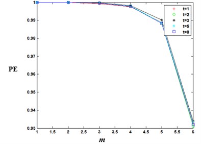
The computation and embedding dimension $q$ of permutation entropy is connected with the value of delay time $t$. Normally the value $q$ has the range of 3-7. If the value $q$ is 1 or 2, at this time, the reconstructed vector contains too few states so that it cannot detect the dynamic mutation of the sequence, and the algorithm loses its validity. If the value of $q$ is too big, the reconstruction of phase space can homogenize the time series, at this time, the calculation is time-consuming and cannot reflect the subtle changes in the series. From the Table 1, we can see that when $q=\text{7}$, the calculation is time-consuming, and the delay time has a little effect on the time series calculation. And from Fig. 1, we can see that delay time $t$ has a little effect on the permutation entropy value of the Gaussian white noise. Therefore, after a comprehensive consideration, this article took $q$ as 6 and $t$ as 1.

Fig. 1Permutation entropy of Gaussian white noise signal at different time delays

4. ELM-AdaBoost algorithm

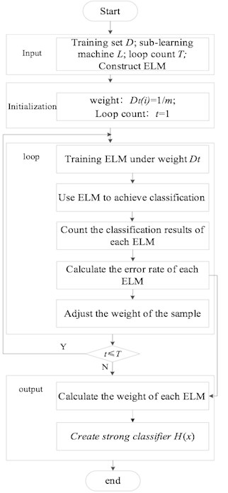
The specific steps of the ELM-AdaBoost algorithm are as follows:

Step 1: Choose $m$ sets of samples from the sample space randomly, by default the sample weights are set as $D_i\left(i\right)=1/m$ to begin the data selection and grid initialization.

Step 2: Choose the ELM to classify the weak classifier. Use the ELM to classify the sample. When training the weak classifier, No.t, use the training sample to train the weak classifier. Additionally, use the training sample to test the weak classifier. Next, calculate an error and ${\epsilon }_t$ of classifier No.t. The calculation formula is as follows:

where $g\left(t\right)$ represents the real prediction classification results, and $y$ represents the expected classification results.

Step 3: Select the weight of the weak classifier. Based on the prediction effects of each ELM (error and ${\epsilon }_t$), calculate each ELM weak classifier weight ${\alpha }_t$. The calculation formula is as follows:

Step 4: Select the sample weight. Renew the weight of the training sample for the next turn according to the weight ${\alpha }_t$ of the ELM weak classifier. Increase the weight of samples with classification errors in this iteration to ensure that the results of these samples can be seen in the next turn. The weight renewal equation is as follows:

where $Z_t$ is the normalization factor.

Step 5: Repeat steps 1 through 4. After $T$ times, the corresponding number of weak classifiers will be successfully created, resulting in the creation of strong classifiers. The weak classifiers are linearly combined with their corresponding weight, and a strong classifier $H\left(x\right)$ is obtained. The equation is as follows:

Fig. 2ELM-AdaBoost algorithm flow chart

5. Experimental study

5.1. Test bench and test system

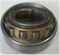
In order to verify the effectiveness of the LCD-MPE and ELM-AdaBoost fault diagnosis methods for train axle box bearing identification, a fault test bench (made by SpectraQuest) was used to simulate bearing faults. As shown in Fig. 3, the bench consists of a driving motor, couplings, gear boxes, and magnetic brakes. The fault test bench simulated 4 bearing conditions: (1) normal bearing conditions, (2) outer race failure conditions, (3) inner race failure conditions, and (4) rolling element failure conditions. In order to simulate failure conditions, we used wire cuts to create slots on the outer race, inner race, and rolling parts. Fig. 4 shows a bearing under all 4 conditions. Under all 4 conditions, the vibration signal sampling frequency was 12k, and the number of sampling points was 4,096. We obtained 20 data sets under each condition, with a total number of 80 samples.

Fig. 3Bearing fault simulation test bench

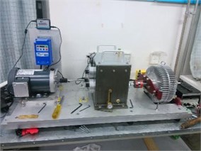
Fig. 44 bearing conditions

a) Normal

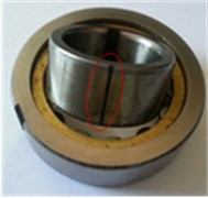
b) Outer race failure

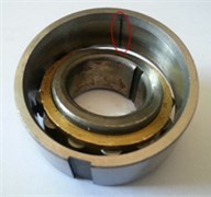
c) Inner race failure

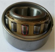
d) Rolling element failure

5.2. Diagnosis results and methodology

With the differences between PE and MPE which were described above, we can realize that MPE can reflect the features of signal in miti-scale because of the scale factor $s$, and the MPE is equal to the PE when $s=\text{1}$, so we choose 4 pieces of vibration signals that represented 4 different states of bearing to calculate their MPE and the deviation of first 5 MPEs. The calculation results are shown in Fig. 5.

As we can see in Fig. 5, the calculation of MPE in first 5 is different from each other, and the deviation of 1st scale MPE which equals to PE is lower than the 2nd and 3rd scale MPE. With this result we can know that MPE has a more powerful feature representation ability. Fig. 6 shows the bearing vibration acceleration of time domain waveforms. Also, since the bearing fault vibration signal amplitude was quite small, it was absorbed by noise. In order to improve the signal-noise ratio (SNR) of the bearing vibration signals, we transformed the wavelets to reduce the noise found in 80 samples of the original data. Fig. 7 shows de-noised signals. By comparing Figs. 6-7, it is evident that after wavelet transformation, some noise components were removed from the original signals, and the SNR of the signals was improved. Fig. 7(a)-(c) clearly shows some periodic impact signal components, but it was difficult to verify the bearing fault type based solely on these impact signals. The LCD method had very good time-frequency locality performance. The LCD method was able to extract the locality information from the bearing vibration signals, and to catch the essential features of the signals. Thus, after the noise reduction, the LCD method was used to decompose bearing vibration signals in all conditions allowed us obtaining several ISCs, as shown in Fig. 8.

Fig. 5First 5 MPEs and their deviation

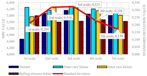
Fig. 6Time-domain waveforms

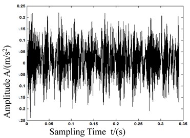
a) Normal

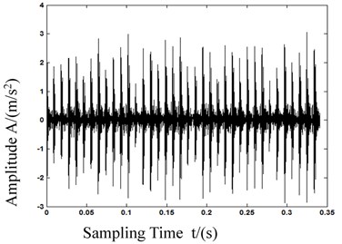
b) Outer race failure

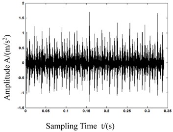
c) Inner race failure

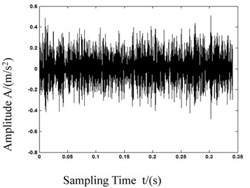
d) Rolling element failure

Each ISC had different time characteristic scales and different energy distributions. From the decomposing results in Fig. 8, it is evident that the bearing fault information was primarily present in the first 5 ISCs.

Fig. 7Waveforms after wavelet transformations

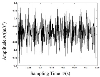
a) Normal

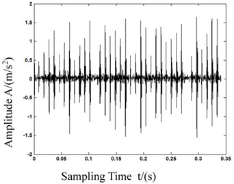
b) Outer race failure

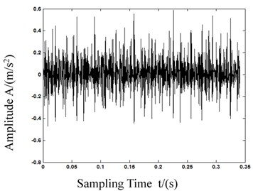
c) Inner race failure

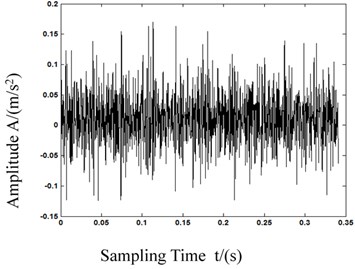
d) Rolling element failure

Fig. 8Waveforms after LCD decomposition

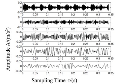
a) Normal

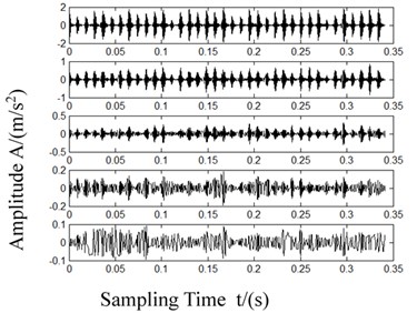
b) Outer race failure

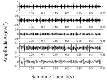
c) Inner race failure

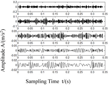
d) Rolling element failure

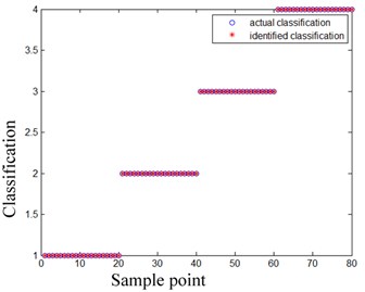
As such, we chose the first 5 ISCs to calculate the multi-scale permutation entropy feature vectors. Fig. 10 shows the MPE feature vectors of the bearings in 4 different conditions. When we calculated the feature vectors, we set the parameter embedded dimension $m$ to 6, delayed the time $t$ to 1, and scaled factor $s$ to 2. Fig. 10 clearly shows that the corresponding MPE feature vectors with different conditions have significant differences. Such evident differences were beneficial for the bearing failure identification. We then calculated the corresponding MPE feature vectors of the remaining groups, and obtained the feature factors of 80 groups. Next, we used the multi-scale permutation entropy results as the feature vectors of the ELM-AdaBoost classifiers. We then chose 5 data groups from each condition (normal bearing conditions, outer race failure conditions, inner race failure conditions, and rolling failure conditions) as the ELM-AdaBoost classifiers training sample, in which numbers 1 through 4 represented normal bearing conditions, outer race failure conditions, inner race failure conditions, and rolling failure conditions, respectively. Finally, the feature vectors are applied as input vectors of SVM and ELM-AdaBoost classifiers to identify a fault. Fig. 11 shows the identification results of SVM classifier, Fig. 12 shows the identification results of ELM-AdaBoost classifier.

From Fig. 11 and Fig. 12, the ELM-AdaBoost model obtains a higher detection rate than SVM for the fault recognition of railway axle box bearings. The experimental results verify that the proposed LCD-MPE and ELM-AdaBoost method is useful for classifying the railway axle box bearings faults considered.

In summary, the LCD-MPE method proposed by us accurately identifies the type of bearing failure.

Fig. 9Permutation entropy under different conditions

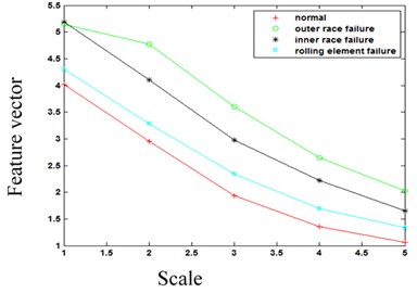
Fig. 10Multi-scale permutation entropy under different conditions

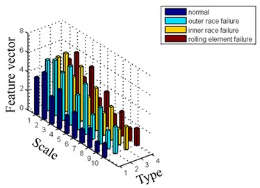
Fig. 11SVM classification results

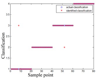
Fig. 12ELM-AdaBoost classification results

6. Conclusions

Based on the non-linear and non-stationary features of train bearing axle box vibration signals, we proposed the LCD-MPE&ELM-AdaBoost fault identification method. We then used our method for the experimental train axle box bearing fault diagnosis. Based on our experiments, we established as follows:

1) LCD is a self-adapted signal processing method that can decompose a complex signal into the sum of finite ISCs. This method is good at processing non-linear and non-stationary signals.

2) Multi-scale permutation entropy (MPE) effectively detects randomness in signals and the dynamic mutations in multiple scales. Moreover, the MPE can extract bearing fault feature information, can create feature sets of bearing vibration signals, and can use the created sets as fault feature information.

3) The ELM-AdaBoost algorithm uses the ELMs as sub-classifiers, combined with the boosting function of the AdaBoost algorithm. It then constructs multi-classification algorithms to solve problems. The ELM-AdaBoost algorithm combined with ELM and AdaBoost accurately identifies train axle box bearing failures in different conditions.

The analysis of normal bearings, outer race, inner race, and rolling part fault signals shows that our proposed method accurately and effectively diagnoses the various fault types of train axle box bearings, what proves our method validity and feasibility. Moreover, the success of our method establishes a theoretical basis for the dynamic monitoring and fault diagnosis of rotating machinery.