Intelligent identification method for whole aero-engine connection stiffness

2.1. Method introduction

The overall calculation flow diagram of the intelligent identification method presented in this study is shown in Fig. 1 mainly divided into the following steps:

1) The initial dynamic model is established. The structure of the whole machine is analyzed to estimate the range of the connection stiffness values.

Fig. 1The overall framework and flow chart of the method

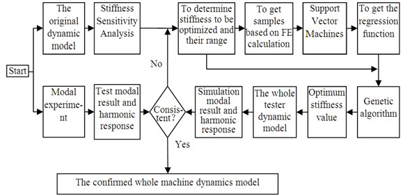
2) The sensitivity analysis of the connection stiffness values on the natural frequencies of the whole machine is conducted.

3) According to the results of sensitivity analysis, the high sensitivity stiffness parameters are selected to be identified.

4) The finite element models are calculated to obtain the corresponding modal frequencies under different stiffness combinations, and form sample sets which are formed by stiffness values combinations and corresponding modal frequencies.

5) For a sample set, the support function vector regression is used to obtain the explicit function relationship between the stiffness values and the modal frequencies of the whole machine.

6) The genetic algorithm is used to identify the stiffness values. The reciprocal of the sum of the absolute values of the differences between the calculated frequencies and the modal frequencies (obtained by the modal test) is set to the fitness function.

7) Finally, the obtained stiffness values are substituted into the whole machine dynamic model for the finite element calculation, and the results are compared with the mode test ones to verify the intelligent identification method.

2.2. Regression function obtained based on SVM

The support vector regression is used to train the sample data to get the prediction model of the stiffness values to the natural frequencies. The model can be extended and perfected by the supplement of the sample.

For a given training sample $\left\{\left({\mathbf{x}}_{\mathbf{i}},{\mathbf{y}}_{\mathbf{i}}\right),i=\mathrm{1,2},...,n\right\}$, ${\mathbf{x}}_i$ as the input vector, and ${\mathbf{y}}_i$ is the corresponding output vector. A non-linear mapping ($\varphi$) is used to map the input vector to a high-dimensional feature space by SVM. And the linear regression is conducted, the regression function is:

Among them, $\mathbf{w}$ and $b$ are weight vectors and thresholds, respectively. $\mathbf{w}•\varphi \left(x\right)$ is the inner product of $\mathbf{w}$ and $\varphi \left(x\right)$, and satisfies the structural risk minimization principle.

The extremum of the objective function is obtained:

Among them, $C$ is the penalty factor to achieve a compromise between the empirical risk and the confidence range. $\epsilon$ is an insensitive function to ensure the sparseness of the dual variables, while ensuring the existence of the global minimum solution and the optimization of the reliable generalization bound. ${\xi }_i$ and ${\xi }_i^{*}$ are relaxation variables solved for $\mathbf{w}$, $b$.

Using the Lagrangian function, Eq. (2) can be transformed into the dual form of solving the Lagrangian operator ${\alpha }_i$, ${\alpha }_i^{*}$. Similar to the classification problem, the kernel function $K({\mathbf{x}}_i,{\mathbf{x}}_j)$ is used to replace the inner product, and the mapping from a low dimensional space to a high dimensional space is realized, thus the nonlinear problem in a low dimensional space is transformed into the linear problem in a high dimensional space. After introducing the kernel function, the optimization objective function becomes as follows:

The corresponding predictive function becomes:

The regression model of SVM can be constructed directly using the Eq. (4).

The support vector regression method based on the structural risk minimization both takes into account the fitness of the training samples, and takes into account the complexity of the training samples, and has a good predictive ability. With a reasonable range of values, the SVM model can approximate the nonlinear function accurately without using much training samples.

2.3. Intelligent recognition based on genetic algorithm

Genetic algorithm was firstly used in the system identification by Goldberg. Since the 1990s, the genetic algorithm application has become more and more extensive. The genetic algorithm application in the system identification is based on the prior knowledge of the specific system, and the genetic algorithm is used as the global optimization method to identify the system parameters by solving the optimization problem.

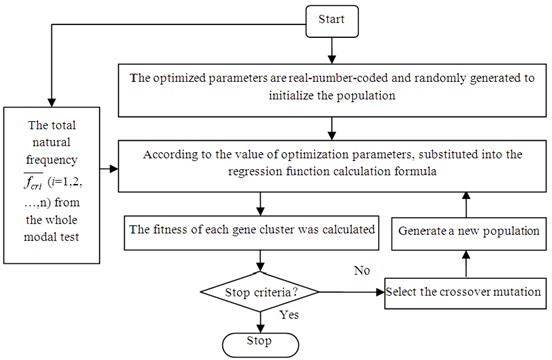
The basic principle of connection parameters identification for a structural system is to optimize them to the objective function, and the objective function is set to the reciprocal of the difference between predictive values and measured values of the modal frequencies of the structural system, and finally the connection parameters are identified. The connection stiffness values identification method based on the genetic algorithm is shown in Fig. 2, the specific steps are:

1) Coding: The selected optimization parameters are: $k_1$, $k_2$,..., $k_n$, using the real number encoding method. The key factor of real number coding is to determine the ranges of each parameter. The appropriate scope will greatly reduce the search space of genetic algorithm, and improve the recognition accuracy and computational efficiency.

2) Fitness function design: target frequency is$\overline{f_{cri}}$, the predicted frequency is $f_{cri}$, $i=$ 1, 2, ..., $n$. The fitness function of the genetic algorithm is defined as:

3) Selection: Using the proportion selection algorithm, i.e. the choice of gambling selection, while using the optimal preservation strategy. Individuals with the highest fitness in the current population do not participate in the crossover and mutation operations, but replace the individuals with the lowest fitness due to the genetic manipulation such as crossover and mutation. Let us suppose that the population size is $M$, and the fitness of individual $i$ is $F_i$, then the probability $p_{is}$ of the individual $i$ is selected as follows:

4) Crossover: Arithmetic crossover method, assuming that the arithmetic crossover is conducted between the two individuals $X_A^t$, $X_B^t$, and, after the cross operation, two new individuals are generated:

Among them, $\alpha$ is the parameter, if $\alpha$ is a constant, using the uniform cross, if $\alpha$ is a variable, the non-uniform cross is used. Here choose $\alpha =$ 0.1, and the uniform cross is used.

5) Variation: Using uniform variation, assume that a gene in the chromosome $x^k$ is the variation point, the value range is [$U_{min}^k$, $U_{max}^k$]. After the uniform variation operation of this chromosome at this point, the new gene is:

In Eq. (8), $r$ is a random obeying [0, 1] evenly distributed.

6) Other parameters: the population is set to 100, the crossover rate is 0.9, and the mutation rate is 0.1.

Fig. 2Genetic algorithm modal recognition process

3.1. Machine mode test

3.1.1. Rotor tester

The research object is an aero-engine rotor tester, which is designed and manufactured by the Shenyang Aero-engine Research Institute. The tester is similar to a real aero-engine by its shape, but the size is reduced to the original one-third. The internal structure is simplified. The shaft is a solid rigid shaft. The test machine is driven by a motor, which constitutes a typical single-rotor aero-engine system model. The true picture of the tester is shown in Fig. 3(a), and its sectional view is shown in Fig. 3(b).

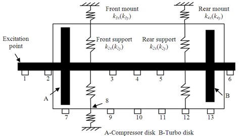
The aero-engine rotor tester is rigidly mounted and fixed on a test platform. The front mounting is located on the left and right sides of the compressor casing, and is fixed to the bracket with bolt structure. The rear mounting section is located on the left side of the turbine stator casing, and the rear section of the tester is suspended by a hinge. The installation section is not symmetrical, resulting in horizontal and vertical dynamic characteristics are not symmetrical, in order to get complete modal results, the modal test should be conducted at horizontal and vertical directions respectively.

Fig. 3Aero-engine rotor tester

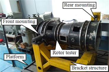
a) Actual aero-engine rotor tester

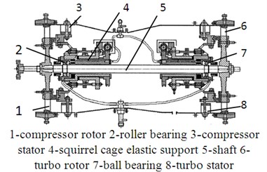
b) Rotor tester profile

3.2. Program

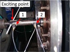
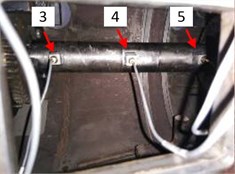
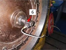
In this study, 13 measuring points are selected for a test, the B&K4508 ICP acceleration sensors are arranged in turn, where 6 measuring points are located at the rotor, and 7 measuring points are located at the stator (the position of the measuring points is shown in Fig. 4). The sine excitation method is used in the test, and the measuring point 1 is the excitation point. The sinusoidal excitation force is measured by an impedance head mounted between the exciter ram and the structure. The modal tests were carried out in the horizontal and vertical directions respectively, and the modal parameters in each direction are obtained.

Fig. 4Scheme of tester modal experiment in horizontal direction

a) Scheme of excitation and measure points position

b) Measurement point 6

c) Measurement point 3-5

d) Measurement point 1-2

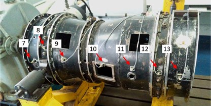
e) Measurement point 7-13

3.2.1. Test results

The modal parameters of first three orders in the horizontal direction (listed in Table 1) can be obtained using the vibration modal identification software; modal shapes are shown in Fig. 5. In Fig. 5, the modal stator shape is presented on the upper half, and the lower half shows the modal rotor shape. In the horizontal direction, the first-order natural frequency is 38.20 Hz, the modal shape is the rotor and stator coupling vibration, wherein there are the rotor pitches and stator pitches. The second-order natural frequency is 46.57 Hz, and the modal shape exhibits the rotor translational rigid vibration behavior, the stator vibration is little. The third-order modal shape is rotor bending, the frequency is 113.42 Hz.

According to the experimental results, the first three modal parameters in the vertical direction are obtained, as shown in Table 2, and the modal shapes are shown in Fig. 6. The first-order natural frequency is 28.84 Hz, the modal shape is rotor pitching, the turbine displacement is larger, and the node position is close to the compressor. The second order is also the rotor rigid vibration, the compressor displacement is larger, and the node position is close to the turbine, the frequency is 42.88 Hz. The third-order modal shape is the rotor bending, frequency is 114.96 Hz. In the first three modes in the vertical direction, the stator has little vibration.

Table 1Experimental modal results in horizontal direction

Order	1st	2nd	3rd
Natural frequency / Hz	38.2	46.57	113.42
Damping ratio	0.0113	0.0167	0.0134

Table 2Experimental modal results in vertical direction

Order	1st	2nd	3rd
Natural frequency / Hz	28.8	42.88	114.96
Damping ratio	0.0114	0.0205	0.0123

Fig. 5First 3 orders modal shapes of rotor tester in horizontal direction

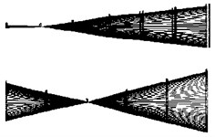
a) 1st order (38.20 Hz)

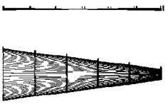
b) 2nd order (46.57 Hz)

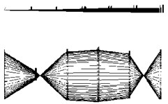
c) 3rd order (113.42 Hz)

Fig. 6First 3 orders modal shapes of rotor tester in vertical direction

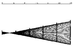
a) 1st order (28.80 Hz)

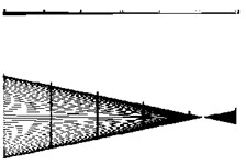
b) 2nd order (46.57 Hz)

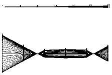
c) 3rd order (114.96 Hz)

The stator-casing thickness of the rotor tester is 4 mm, which implies that the stator stiffness is high. The phenomenon of coupling vibration of the stator and rotor in the horizontal direction is not caused by their structures alone. The stator vibration in the horizontal direction is due to the mounting method. The rear tester mounting is a hanging hinge that lifts the tester tail, implying that the rear tester side is not constrained in the horizontal direction. Hence, the rigid modal shape of the first order stator and rotor coupling is due to the mounting method of the tester.

3.3. Identification of whole tester stiffness

3.3.1. Whole tester stiffness analysis

1) Finite element modeling.

The structure of the rotor tester is complex. There are observation holes, excitation holes, bolts, keyways and other small size structures on the casing, these structures have a little effect on dynamic characteristics. However, these structures will increase the scale of the finite element model when meshing the geometrical model, which increases the computation steps. Hence, the structure is simplified for the modeling process, and some small-size structures are neglected. Tester rotor material is 30CrMnSi, the casing material is 1Cr18Ni9Ti. The material parameters are shown in Table 3.

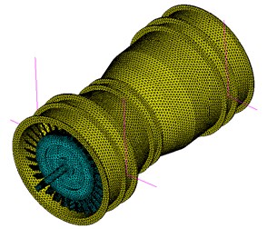
Fig. 4(a) shows the position of mountings and supports. $k_{1x}$, $k_{1y}$ are the horizontal and vertical stiffness of the rotor front supports, respectively. $k_{2x}$, $k_{2y}$ are the horizontal and vertical stiffness of the rotor rear supports. $k_{3x}$, $k_{3y}$ is the horizontal and vertical stiffness of the front mounting. $k_{4x}$, $k_{4y}$ is the horizontal and vertical stiffness of the rear mounting. SOLID186 is selected to mesh the rotor and stator structures, and Conbin14 is selected to simulate the bearings. The finite element model is shown in Fig. 7. There are 179763 units and 57204 nodes.

Table 3Material parameters of tester model

Elastic modulus / (Pa)	Density / (kg/m3)	Poisson’s ratio
2.11×1011	7800	0.3

Fig. 7Finite element model of whole rotor tester

2) Structural analysis and stiffness range estimation.

The tester has a total of four stiffness parameters. $k_1$, $k_2$ is the rotor supports stiffness, and $k_3$, $k_4$ is the mountings stiffness. The rotor is supported by an elastic squirrel cage support structure in series with the bearing structure. The rigidity of squirrel cage support structure is weak and plays a major role in series stiffness. The bearing in a front support (support 1) is a cylindrical roller bearing, the bearing designation is N206EM. The rear element in rear support (support 2) is a deep groove ball bearing, the bearing designation is 6206. According to the experience, simulation and modal test results, the range of $k_{1x}$, $k_{1y}$, $k_{2x}$, $k_{2y}$ is from 1×10⁵ N/m to 2×10⁶N/m. The front mounting is fixed at the bracket with a ball-winch structure. Its horizontal and vertical stiffness is strong; the range of $k_{3x}$ and $k_{3y}$ is from 5×10⁶ N/m to 5×10⁷N/m. The rear mounting is hinged vertically in one side. The stiffness of rear mounting in the horizontal direction is weak. The range of k_4x is considered from 1×10⁶ N/m to 5×10⁶N/m. The stiffness in the vertical direction is stronger than the one in the horizontal direction, and the range of $k_{4y}$ is 5×10⁶ N/m-5×10⁷N/m.

3) Analysis of influence of stiffness on natural frequencies.

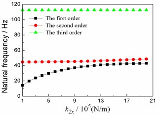
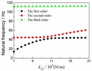
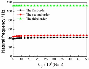
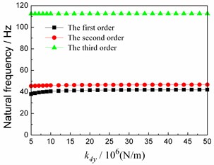
$k_{1x}$, $k_{1y}$, $k_{2x}$, $k_{2y}$ are set to 1×10⁶N/m, $k_{3x}$ and $k_{3y}$ are equal to 1×10⁷N/m, $k_{4x}$ is 5×10⁶N/m, $k_{4y}$ is 5×10⁷N/m. By changing one of the stiffness values alone and calculating the first three natural frequencies, the influence of the changed stiffness on the first three natural frequencies can be obtained. As the horizontal and vertical stiffness is not symmetrical, the first three natural frequencies in the horizontal and vertical directions are calculated respectively. The results are shown in Fig. 8 and Fig. 9.

It can be seen from Fig. 8 that the first two natural frequencies in the horizontal direction are strongly affected by $k_{1x}$, $k_{2x}$ and $k_{4x}$ and are not sensitive to the change of $k_{3x}$. When $k_{3x}$ is greater than 1×10⁷ N/m, the natural frequency of each order is not changed any more. The third-order natural frequency in the horizontal direction is not affected by the change of stiffness. Therefore, the horizontal direction selection $k_{1x}$, $k_{2x}$ and $k_{4x}$ are the preferred optimization parameters.

It can be seen from Fig. 9 that the natural frequencies of the first two orders in the vertical direction are greatly affected by $k_{1y}$ and $k_{2y}$, and are affected a little by $k_{3y}$ and $k_{4y}$. Among them, the impact by $k_{3y}$ is smaller. When $k_{3y}$ is greater than 1×10⁷ N/m, the natural frequency of each order is not changed any more. And the third-order natural frequency in the vertical direction is not affected by the change of stiffness. In summary, $k_{1y}$, $k_{2y}$ and $k_{4y}$ are selected to be the optimum stiffness in the vertical direction.

Fig. 8Relationship between first 3 orders natural frequencies and stiffness values in horizontal direction

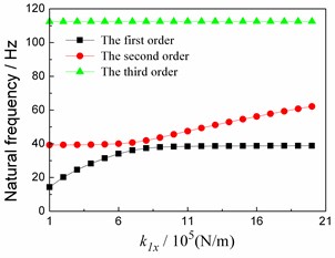
a) Change of $k_{1x}$

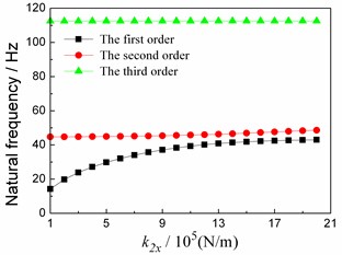
b) Change of $k_{2x}$

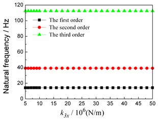
c) Change of $k_{3x}$

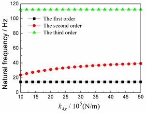
d) Change of $k_{4x}$

Fig. 9Relationship between first 3 orders natural frequencies and stiffness values in vertical direction

a) Change of $k_{1y}$

b) Change of $k_{2y}$

c) Change of $k_{3y}$

d) Change of $k_{4y}$

4) Sample calculation.

It is found that the horizontal stiffness parameters only affect the natural frequencies in the horizontal direction, while the vertical stiffness values only affect the natural frequencies in the vertical direction. So, the horizontal direction and the vertical direction are optimized separately.

As previously described, for the horizontal direction, $k_{3x}=$ 1×10⁷N/m, the range $k_{1x}$, $k_{2x}$ is from 1×10⁵ N/m to 2×10⁶N/m, $k_{4x}$ is from 1×10⁶ N/m to 5×10⁶N/m. In the ANSYS software, the first three natural frequencies ($f_{H1}$, $f_{H2}$, $f_{H3}$) shall be calculated in the horizontal direction under different $k_{1x}$, $k_{2x}$, $k_{4x}$ values combinations. A set of samples is constructed consisting of $k_{1x}$, $k_{2x}$, $k_{4x}$ and $f_{H1}$, $f_{H2}$, $f_{H3}$ respectively. Similarly, for the vertical direction, $k_{3y}=$ 1×10⁷N/m, the range of $k_{1y}$, $k_{2y}$ is from 1×10⁵ N/m to 2×10⁶N/m, the range of $k_{4y}$ is from 5×10⁶ N/m to 5×10⁷ N/m.

$f_{H1}$ is an example to illustrate the sample construction method: every calculation, a four-dimensional vector, that is, a sample point, which constitutes by $k_{1x}$, $k_{2x}$, $k_{4x}$ and $f_{H1}$, can be obtained. A set of sample points for all combinations of values within the range can be used as a training sample for SVR modeling.

In model training and testing, the total samples are randomly divided into a half as training samples, and the others are as the test samples. In calculation, because the number of the parameters in a range is endless, for a parameter, some values in its corresponding range are selected for a calculation. In calculation, 75 sample points are obtained for each order natural frequency in one direction. The sample data are collated to form sets of samples, which combine the stiffness value combination and its corresponding modal frequency.

3.3.2. Intelligent identification of whole test connection stiffness

1) Regression function of stiffness values to natural frequencies based on SVR.

Based on the SVR technique, the mapping of the natural frequency to stiffness values is obtained. The mapping reflects the functional relationship between the input (connection stiffness) and the output (natural frequency) of the finite element model.

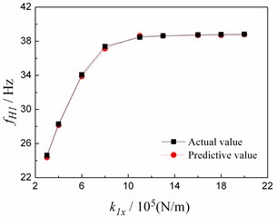
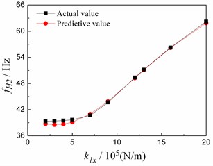
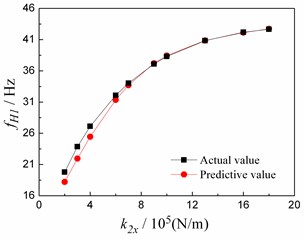
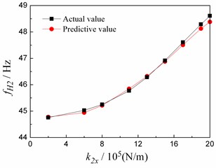
The first two orders of natural frequency data are used to carry out the support vector regression prediction test, Fig. 8 shows the results. Among them, samples 1-4 characterize the relationship between $k_{1x}$ and $f_{H1}$, $k_{1x}$ and $f_{H2}$, $k_{2x}$ and $f_{H1}$, and $k_{2x}$ and $f_{H2}$, respectively. The support vector parameters of samples are identified by the genetic algorithm, as shown in Table 4, and the test results are shown in Fig. 10.

Table 4Support vector parameters and mean square error

Sample number	$\gamma$	$C$	eps	Mean square error / %
1	1.0138	343.999	0.1	0.71
2	0.7666	345.664	0.1	0.82
3	0.0715	292.521	0.1	0.85
4	0.0033	24.4758	0.1	0.89

It can be seen from Fig. 11 that there is a good agreement between the predicted natural frequencies and the actual natural frequencies. The results show that the model has good generalization ability, and it can be used to replace the whole tester finite element calculation. It can be used to predict the natural frequency of the tester.

Respectively, the support vector regression analysis is carried out in the horizontal direction and vertical direction, respectively, so we can get:

9

$\left\{\begin{array}{l}f\left(f_{H1}\right)=f_1\left(k_{1x},k_{2x},k_{4x}\right),\\ f\left(f_{H2}\right)=f_2\left(k_{1x},k_{2x},k_{4x}\right),\end{array}\right.$

10

$\left\{\begin{array}{l}f\left(f_{V1}\right)=g_1\left(k_{1y},k_{2y},k_{4y}\right),\\ f\left(f_{V2}\right)=g_2\left(k_{1y},k_{2y},k_{4y}\right).\end{array}\right.$

Eqs. (9) and (10) are the support vector regression models of the connection stiffness to the natural frequencies in the horizontal and vertical directions, respectively.

2) Stiffness identification based on genetic algorithm.

Based on the natural frequency prediction model, the experimental results are regarded as the target to identify the stiffness values in the horizontal and vertical directions, respectively. In calculation, the number of population and evolutionary algebra are both set to 100. Fig. 11 shows the convergence curves of the fitness values with genetic algebra in the horizontal and vertical directions, respectively. The recognition results are shown in Table 5 and Table 6.

Fig. 10Natural frequency model test results

a) Sample 1

b) Sample 2

c) Sample 3

d) Sample 4

Fig. 11Genetic algorithm convergence curve

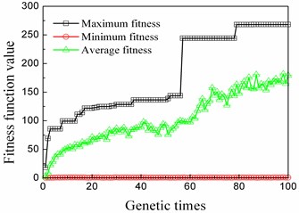
a) Horizontal direction

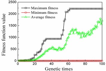
b) Vertical direction

Table 5Horizontal stiffness parameters identification results

$k_{1x}$ / 106N/m	$k_{2x}$ / 106 N/m	$k_{3x}$ / 106 N/m	$k_{4x}$ / 106 N/m
1.1008	1.1208	10	4.1031

Table 6Vertical stiffness parameters identification results

$k_{1y}$ / 106 N/m	$k_{2y}$ / 106 N/m	$k_{3y}$ / 106 N/m	$k_{4y}$ / 106 N/m
0.9408	0.464	10	6.0814

3.4. Results verification

1) Horizontal results validation.

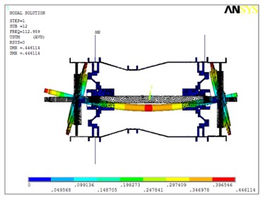
The results in Table 5 are substituted into the finite element model to calculate the first three modes in the horizontal direction, and the modal shapes are shown in Fig. 12. The first-order vibration modal shape is the rigid vibration mode, rotor and stator coupling vibration, wherein there are rotor pitches, stator pitches, and the frequency is 38.23 Hz. The second-order vibration modal shape exhibits the rigid vibration behavior. The performance is the rotor translational motion, the frequency is 46.34 Hz. The third-order vibration mode of the tester is the rotor bending at a frequency of 112.96 Hz. The calculated results agree well with the experimental results.

Fig. 12Simulation first 3 orders modal shapes in horizontal direction

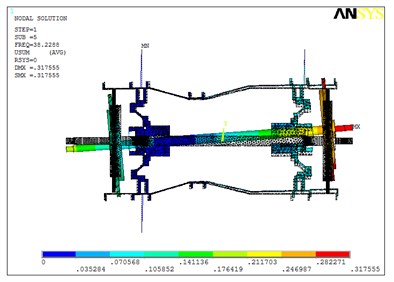
a) First order (38.23 Hz)

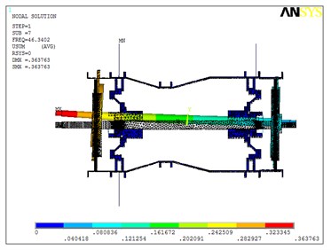
b) Second order (46.34 Hz)

c) Third order (112.96 Hz)

The first three natural frequencies in the horizontal direction are compared with the experimental results, shown in Table 7. The error calculation is based on the test results.

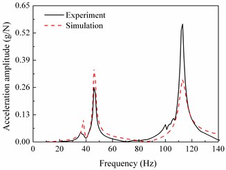
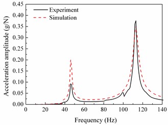
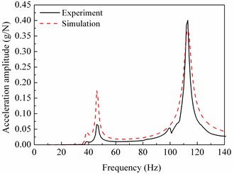
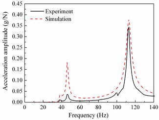
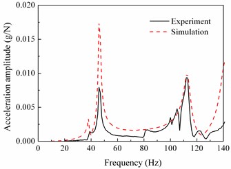
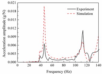
Further, the horizontal harmonic response of the simulation model is calculated. The simulation acceleration frequency response of each measuring points are compared with the experimental ones. The harmonic response comparisons between simulation and experiment of the measuring points 1, 3, 4, 5, 7 and 10 are shown in Fig. 13.

From Fig. 12, Fig. 13 and Table 7, the following conclusions can be drawn:

1) The first three order modal shapes obtained from the simulation and the experiment are similar in the horizontal direction. The first-order modal shapes both are the rotor and stator rigid coupling vibration, the second-order modal shapes both exhibit the rotor translational motion, the third-order ones both are rotor bending.

2) The first three-order natural frequencies of simulation are in a good agreement with the experimental results. The maximal relative error between the simulation and test of the first three-order natural frequencies is only –0.49 %.

3) The simulation acceleration-frequency response functions strongly coincide with the experimental ones at the points 1, 3, 4, 5, 7 and 10.

Fig. 13Comparisons between frequency response functions of experiment and those of simulation in horizontal direction

a) Test point 1 (rotor)

b) Test point 3 (rotor)

c) Test point 4 (rotor)

d) Test point 5 (rotor)

e) Test point 7 (casing)

f) Test point 10 (casing)

2) Vertical results validation.

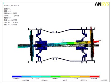
The results in Table 6 are substituted into the finite element model to calculate the first three modes in the vertical direction, and the modal shapes are shown in Fig. 14. In the first three order modal shapes, the stators have little vibration. The natural frequency of the first order in the vertical direction is 28.65 Hz, and the modal shape exhibits the rotor pitch behavior. The turbine displacement is larger than the compressor displacement, and the node position is close to the compressor. The second-order natural frequency is 42.69 Hz, the modal shape is the rotor pitch, the compressor displacement is larger than the turbine displacement, and the node is near the turbine. The third-order natural frequency is 114.96 Hz, the modal shape is rotor bending.

The first three natural frequencies in the vertical direction are compared with the experimental results, as shown in Table 8. The error calculation is based on the test results.

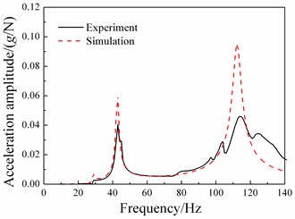
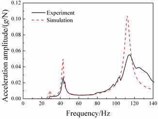
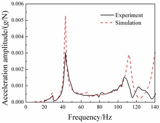
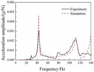
Further, the vertical harmonic response of the simulation model is calculated. The simulation acceleration frequency response of each measuring points are compared with the experimental ones. The harmonic response comparisons between simulation and experiment of the measuring points 1, 3, 4, 5, 7 and 10 are shown in Fig. 15.

Fig. 14Simulation first 3 orders modal shapes in vertical direction

a) 1st order (28.84 Hz)

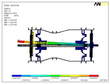
b) 2nd order (42.88 Hz)

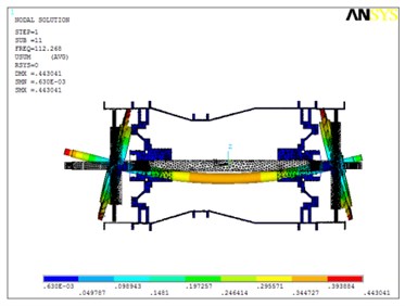
c) 3rd order (114.96 Hz)

From Fig. 14, Fig. 15 and Table 8, the following conclusions can be drawn:

1) The first three-order modal shapes obtained from the simulation and the experiment are similar in the vertical direction. The first-order modal shapes both demonstrate the rotor and stator rigid coupling vibration, the second-order modal shapes both exhibit the rotor translational motion, the third-order ones both are rotor bending.

2) The first three-order natural frequencies of simulation are in a good agreement with the experimental results. The maximal relative error between the simulation and test of the first three order natural frequencies is only –2.34 %.

3) The simulation acceleration-frequency response functions strongly coincide with the experimental ones at the points 1, 3, 4, 5, 7 and 10.

In summary, the modified model can effectively simulate the real characteristics of the tester. Both the horizontal and vertical stiffness parameters obtained by the intelligent method can be used to characterize the connection stiffness of the tester. The recognition method is correct, and the recognition results are reliable. In this method, the genetic algorithm can be replaced by other algorithms.

Fig. 15Comparisons between frequency response functions of experiment and those of simulation in vertical direction

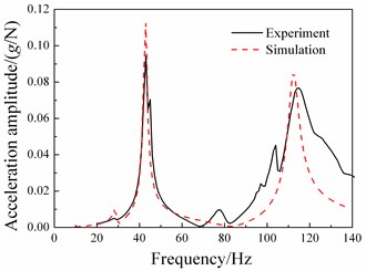
a) Test point 1 (rotor)

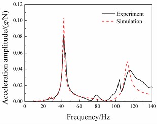
b) Test point 3 (rotor)

c) Test point 4 (rotor)

d) Test point 5 (rotor)

e) Test point 7 (casing)

f) Test point 10 (casing)