A hydraulic fault diagnosis method based on sliding-window spectrum feature and deep belief network

2.1. The DBN structure

A DBN is a feedforward neural network stacked with several Restricted Boltzmann Machines (RBMs), which consists of a visible layer, a number of hidden layers, and an output layer [15]. As shown in Fig. 1, a DBN with four layers is taken as the example to introduce the principle of DBN. This DBN includes two unsupervised RBMs and one supervised BP classifier. In the DBN, the visible layer used to accept input data and the 1st hidden layer compose the RBM1, the 1st and 2nd hidden layers compose the RBM2, and the 2nd hidden layer and the output layer compose the BP classifier.

Fig. 1Structure diagram of a DBN with two hidden layers

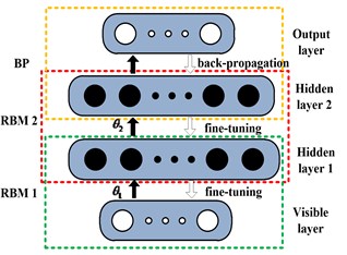
The DBN training process consists of two parts, including unsupervised training and supervised training. In the unsupervised training part, the entire network parameters are initialized firstly, and then the RBMs are trained through greedy algorithm. After the training of last RBM is completed, the output of its hidden layer is taken as the input of visible layer of next RBM, and by thus layer-by-layer training, the parameters of each RBM are acquired. In the supervised training part, the label layer of data is brought into training process. The training error is distributed to each RBM by BP classifier through back-propagation algorithm, thereby realizing the updating of the parameters.

2.2. The training process of RBM

RBM is a special kind of Markov random field, as well as an energy-based stochastic neural network [16], its energy function of visible layer $v$ and hidden layer $h$ can be defined as:

where $v_i$ and $h_j$ are the binary state of visible unit $i$ and hidden unit $j$, $w_{ij}$ is the weight between them, $a_i$ and $b_j$ are the biases of corresponding units.

Each RBM has one visible layer and one hidden layer, for the two layers, all the visible units and hidden units are connected to each other symmetrically and bidirectionally, and there is no connection between any two units within the same layer. Any of the unit state can be either 1 or 0. The joint probability distribution of visible layer$v$ and hidden layer$h$, and the conditional probabilities of visible unit$v_i$ and hidden unit $h_j$ can be given as:

where $W$ is the weight matrix between visible unit and hidden unit, respectively $a$ and $b$ are the biases matrix of corresponding units.

Researches from experts like Hinton have proved that the parameters $\theta =\left\{W,a,b\right\}$ making $p\left(v,h\right)$ maximized can be obtained by Contrastive Divergence (CD) algorithm. According to CD algorithm, the update rule of the RBM parameters $\theta =\left\{W,a,b\right\}$ is:

where ${\epsilon }_W$, ${\epsilon }_a$, ${\epsilon }_b$ are learning rate of weight, biases of hidden layer and visible layer. ${〈\bullet 〉}_{data}$ refers to the expectation decided by the probability distribution of training data, and is easy to calculate its unbiased estimation. ${〈\bullet 〉}_{recon}$ refers to the expectation decided by the probability distribution of reconstructed data. $m$ is the inertiafactor, which associates the anteroposterior update parameters, and is used to keep the stability of parameter updating.

2.3. The advantages of DBN

A large number of experiments prove that, compared with the traditional BP neural network, DBN doesn’t need many labeled training samples, and is no longer limited to the effect of random initialization. RBM is trained layer-by-layer through unsupervised and greedy training, and the training result is taken as the initial value of probability model of supervised learning. This approach can speed up the convergence speed of network, solve the problem of tending to fall into local optimal of BP neural network, improve the learning ability, and provide a technical support for the efficient and deep learning.

3.1. Problems of applying characteristic spectrum

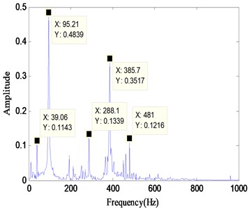
The spectrum curve of vibration signal contains the system’s state information, when the state varies, the spectrum would also change. Spectrum curve is actually a multimodal function, which usually consists of multiple local peaks [17]. As shown in Fig. 2, the spectrum curve of a hydraulic signal taken from the article’s experiment set, contains nearly 10 significant local peaks. Actually, each local peak is corresponding to a vibration mode. Therefore, in view of the signal’s generation mechanism, a local peak should be a complete feature. In one local peak, pick out the spectrum of maximum amplitude, and define its frequency as the characteristic spectrum of this local peak, such as the frequency of 95.21 Hz in Fig. 3. Obviously, a characteristic spectrum is a vibration mode, and a local peak can be considered as a frequency band decided by the certain characteristic spectrum, and the frequency bands vary in width.

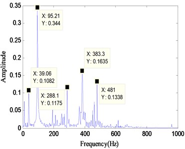
In the fault diagnosis based on vibration testing technology, the spectrum is often taken as the input features of classifier. In reference [18], the whole Hilbert envelope spectrum of bearing fault signals are used as the feature vectors of DBN, which may cause the following defects. For example, the frequency band containing characteristic spectrum would be dismembered, which destroys the completeness of feature. And make the dimension of input vector very high, which would add the burden of classifier and increase the running time. Besides, for the same type of test sample, there is the risk of relative shifting of characteristic spectrum. For example, Fig. 3 shows the spectrogram of two samples of the same type, judging from the significant frequencies of the two figures, the frequencies of 383.3 Hz and 385.7 Hz should be the representation of the same fault feature. However, the relative shifting of characteristic spectrum appears as a result of test environment or man-made factors, which would have a negative impact on the subsequent classification process.

Fig. 2The spectrum curve of a hydraulic signal

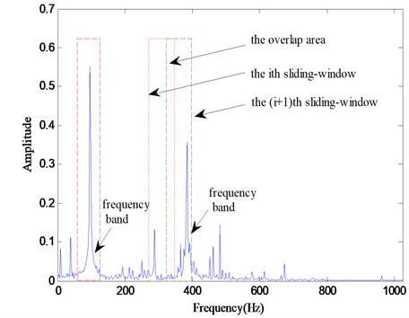
Fig. 3The relative shifting of characteristic spectrum in different samples

a)

b)

Obviously, the division of spectrum curve should be an effective method for above defects. Krakovsky [19] uses the moving-window discrete Fourier transform as a multichannel filter. Ye [20] do the modal decomposition by segmenting the spectrum curve. And Ma [21] uses sliding window FFT algorithm to analysis low frequency oscillation. These papers mainly utilize sliding window for modal analysis or frequency filter, and they split the spectrum function directly into several fragment. But in this paper, the sliding method is used as a feature extraction approach and takes the overlap rate into account. Ideally, by dividing each frequency band corresponding to the characteristic spectrum should be well separated, and these frequency bands would be used as feature vectors. In this case, the integrity of characteristic frequency band is kept, the relative shifting of characteristic spectrum avoided and the dimensions of feature vectors reduced. If adopting the method of equidistant division, it would be difficult for the complete characteristic frequency band to avoid being broken down. If using the method of artificial division, the workload would be increased greatly.

3.2. Specific steps of SWSF method

Therefore, in this article, the way of sliding for division is adopted and a feature extraction method based on sliding-window spectrum feature (SWSF) is proposed. The specific steps are as follows.

Step 1, perform spectrum transform for vibration signal $x\left(t\right)$. In this article, calculate the Hilbert envelope spectrum of $x\left(t\right)\text{,}$ and take its unilateral spectrum sequence $F\left(\omega \right)\text{.}$ The subsequent dealing objects are pointing at $F\left(\omega \right)$.

Step 2, determine the width $W$ of sliding-window and the overlap rate $O$ of adjacent sliding-windows, and ensure that the product of $W$ and $O$ is an integer (see Fig. 2).

Step 3, the abscissae of starting and ending of the first sliding-window can be given as:

Sum up spectrum sequence of $F\left(\omega \right)$ in the first sliding-window, and get the first sliding spectrum feature $H\left(1\right)$:

Step 4, conduct the $i$th sliding. Judge whether the ending abscissa of the last sliding is not greater than the sequence length of $F\left(\omega \right)$. If not, the loop terminates. Otherwise, continue sliding. At the moment, the abscissae of starting and ending of the $i$th sliding-window can be given as:

Sum up spectrum sequence of $F\left(\omega \right)$ in the ith sliding-window, and get the $i$th sliding spectrum feature $H\left(i\right)$:

Step 5, obtain the new feature sequence $H\left(v\right)$ of sliding spectrum.

By the feature extraction process SWSF for vibration signal, the feature sequence $H\left(v\right)$ is obtained, which is similar to the histogram sequence in statistical method (hereinafter referred to as sliding spectrum).

The Hilbert envelope spectrum is adopted in the SWSF method, its process can be given as:

1) Perform the Hilbert transform for signal $x\left(t\right)$:

2) Calculate the envelope signal $e\left(t\right)$:

3) Carry on Fourier transform for the envelope signal $x\left(t\right)$, select its unilateral spectrum sequence $E\left(f\right)$ as the envelope spectrum of signal $e\left(t\right)$:

3.3. An example of applying SWSF

The feature extraction process SWSF is performed for a hydraulic signal under the sliding width of 2 and 4, and overlap rate of 0 respectively. According to the result shown in Fig. 4, the dimensions of sliding spectrum reduce significantly, which are 512 and 256, compared with the 1024 dimensions of the signal’s Hilbert envelope spectrum.

4.1. Experiment introduction

The vibration signals used in this paper are measured on the synthetical hydraulic fault experimental platform as shown in Fig. 5, which is entirely made of steel. And these signals are respectively tested under the five states of normal, blockage, leakage, cavitation and impulsion. The measuring points are distributed on the hydraulic cylinder, the sampling frequency is 5000 Hz and the number of sampling points is 2048. Fig. 6 illustrates the time-domain graphs of signals in normal and other four failure states. The figure indicates that the tested vibration signals present different variation rule with different working states, but it is not enough to distinguish these states just depending on the time domain analysis.

Fig. 4Sliding spectrums in two cases

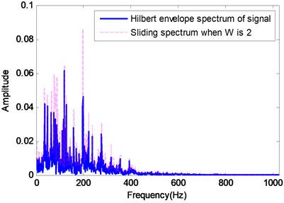
a) When $W$ is 2

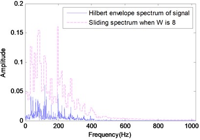
b) When $W$ is 8

Fig. 5The synthetical hydraulic fault experimental platform and its schematic diagram. 1 – fuel tank, 2 – suction filter, 3 – control valve of oil-absorbing blockage, 4 – control valve of cavitation, 5 – hydraulic pump, 6 – electromotor, 7 – piezometer, 8 – relief valve, 9 – hand-directional valve, 10 – control valve of leakage, 11 – one-way throttle valve, 12 – flowmeter, 13 – control valve of oil inlet blockage, 14 – control valve of oil outlet blockage, 15 – hydraulic cylinder, 16 – clamping sleeve, 17 – load

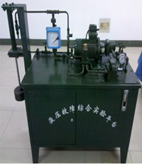
a)

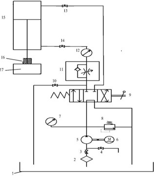
b)

4.2. Analysis of experiment results

To validate the proposed hydraulic fault diagnosis method combining SWSF and DBN, the data tested from the synthetical hydraulic fault experimental platform is used as the experiment sample set. The training set is consist of 300 samples in normal state, 300 in blockage, 300 in leakage, 300 in cavitation and 180 in impulsion, totaling 1380 samples. And the corresponding testing set is made up of 200 samples in normal state, 200 in blockage, 200 in leakage, 200 in cavitation and 100 in impulsion, totaling 900 samples. Before diagnosis of the experiment sample set, the main structure parameters of DBN need to be determined, and then situations in different sliding width and overlap rate. During the discussing process, the evaluation criteria mostly depend on testing accuracy, while allowing for the elapsed time flexibly.

Fig. 6Time-domain plots of hydraulic vibration signals in five different states

a)

b)

c)

d)

e)

4.2.1. Discussion on the main structure parameters of DBN

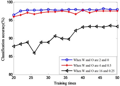
The structure of adopted DBN is $M$-$n$-$n$-5, where $M$ is the dimension of input data, $n$ is the number of units in the hidden layer which usually vary from 10 to 100, and the 5 represents 5 types of states. Obviously, $n$ is an important parameter to for DBN, besides, training times of DBN has a great effect on the classification accuracy and consuming time. Thus, the n and training times are discussed in the following three cases, when the $W$ and $O$ are 2 and 0, 4 and 0.5, 16 and 0.25 respectively.

1) Discussion on the number of hidden units.

When discussing about the value of the number n of hidden units, define the training times as 50 firstly. Then repeating classification testing 10 times, get the averages of these testing results shown in Table 1. By comparison，it is found that the classification accuracy is more better when the number of hidden units is 100, therefore, 100 is decided as the value of n finally.

Table 1Classification results of the DBN with different hidden units

Classification accuracy (%)	Number of hidden units
	20	40	60	80	100	20
$W/O$	2/0	93.11	94.56	97.56	97.78	98.00
	4/0.5	92.56	96.89	96.00	97.33	97.33
	16/0. 25	89.56	89.78	90.00	90.22	91.56

2) Discussion on training times.

According to the previous result, when discussing the training times, choose 100 hidden units and repeat classification testing 10 times. The averages of testing results are displayed in Fig. 7. Combined with the three cases, the curves of classification accuracy tend to be smooth after training times reaches 40. Because the consuming time of DBN’s diagnosis is positive correlated with the training times, so 40 is confirmed as the final value of training times.

Based on the above discussion results, finally, the network structure of DBN can be given as M-100-100-5, and the training times is 40.

Fig. 7Classification results with different training times

4.2.3. Change process of features in DBN

In order to study the change process of the feature in each layer of DBN, the input data and output data of two hidden layers are disposed by the principal component analysis (PCA) method. For an alternative visualization, the 3D plots of the first three principal components are shown in Fig. 8, when sliding width is 3 and overlap rata is 0. Fig. 8(a) indicates a poor aggregation with the mixing of a great part features of the 5 states. After the first hidden layer, as shown in Fig. 8(b), there are significant differences between features in each state, except for that between leakage and impulsion, besides a slight mixing is exist between normal and blockage. After the second hidden layer (Fig. 8(c)), in addition to the mixing of a few features between leakage and impulsion, the aggregation extent and the difference between each state improve greatly. The above result suggests that through the feature extracting in hidden layers of DBN layer by layer, the distribution of feature is greatly optimized, the expression ability improved and the discrimination enhanced, thereby performing the following state classifying effectively.

Fig. 8The first three principal components of testing samples

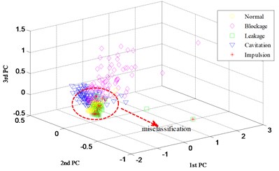
a) Input data

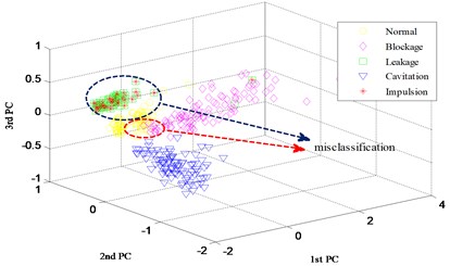
b) Output of the 1st hidden layer

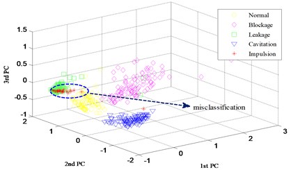
c) Output of the 2nd hidden layer