Abstract
Assumptions accompanying exponential failure models are often not met in the standard sequential probability ratio test (SPRT) of many products. However, for most of the mechanical products, Weibull distribution conforms to their life distributions better compared to other techniques. The SPRT method for Weibull life distribution is derived in this paper, which enables the implementation of reliability compliance tests for gearboxes. Using historical failure data and condition monitoring data, a life prediction model based on hidden Markov model (HMM) is established to describe the deterioration process of gearboxes, then the predicted remaining useful life (RUL) is transformed into failure data that is used in SPRT for further analysis, which can significantly save on testing time and reduce costs. Explicit expression for the distribution of RUL is derived in terms of the posterior probability that the system is in the unhealthy state. The predicted and actual values of the residual life are compared, and the average relative error is 3.90 %, which verifies the validity of the proposed residual life prediction approach. A comparison with other life prediction and SPRT methods is given to elucidate the efficacy of the proposed approach.
1. Introduction
With the rapid development of aviation, high-speed trains, shipbuilding and other industries, reliability compliance tests need to be done for a large number of equipment with new designs or major changes to verify whether the product reliability indexes meet the stipulated requirements and reliability test values, which has the potential to provide improvement measures for development and reasonable criterion for acceptance. Gears, as the key components of mechanical transmission, are widely used in the aviation, energy industry and in heavy machineries such as helicopters, wind turbines and heavy trucks. Therefore, the gear reliability compliance test is particularly important.
Currently, reliability compliance testing schemes include the time-terminated test, fixed-sample test and sequential probability ratio test (SPRT). In reliability compliance tests, the SPRT method can use the test information generated in the process of judgment, so there is no need to test for specified deadlines or failure numbers. In general, compared with other sampling test methods, such as the time-terminated test and fixed-sample test, shorter average cumulative testing time and smaller average failure numbers are required for decision making in SPRT [1, 2]. Under the circumstances of scarce on hand data and the unknown prior distribution for the life of new products, Li et al. [3] established a reliability growth model using small sample data sets based on the SPRT and Bayesian theorem, the results of which indicated that without assuming prior distribution for the new products, the reliability was increased using the proposed method. Shinichiro et al. [4] applied the SPRT to the nervous system. The SPRT chart is also an effective control chart to detect mean shifts in statistical process control [5, 6]. However, the current sequential sampling test method introduced in some standards about SPRT (such as GJB 899A-2009, MIL-STD-781D) assumed that the life of products followed exponential distribution [7, 8], which is not applicable for most mechanical products with depletion-type life. A lognormal distribution was better fit for the fatigue life distribution of certain parts [9]. The two-parameter Weibull distribution is more appropriate to describe the life of some key components, such as rolling bearings and gears [10-12]. Therefore, the reliability compliance test method without the restrictions of the exponential distribution is a research hotspot in recent years. To address this situation, Hauck and Keats [13] pointed out that the Weibull distribution can be transformed to exponential distribution to derive the sequential compliance test plan for Weibull distribution with the accurate estimates of the unknown shape parameters needed. Meanwhile, after transformation, the validation indexes are the qualified life and the limited life , which need to be determined in advance by the given lifetime reliability. With the assumption that the shape parameter was known and the scale parameter was a random variable, Tsai et al. [14] established a fixed-sample test plan for Weibull life type products in the condition of limited test equipment, the reasonableness of which was also verified by case calculation. Pandit and Gudaganavar [15] studied on the SPRT for Gamma distribution and discussed the robustness of the plan when the shape parameter changes. The SPRT for lognormal distribution was derived by Deng and Yuan [16] with the upper and lower limits of the producer’s risks and the consumer’s risks in the truncated sequential test studied. Although many researchers studied SPRT for non-exponential distribution and the actual failure time of products in the tests were utilized to decide whether to accept or reject the products, we note that few literature considered condition monitoring information in the test plans, which are common in practice. Under limited resources, Li et al. [17] made the SPRT decisions with the consideration of life prediction data, but the specific prediction method for residual life was still not given. Such a drawback for Weibull distribution in the existing literature motivates us to improve the SPRT method. Using gears as the research object, we establish the SPRT plan for Weibull distribution in accordance with the actual gear life. Moreover, the historical failure data and the condition monitoring information of current products are used for the accurate life prediction, then judgments can be made under the restrictions of test equipment and costs.
In condition-based maintenance (CBM), vibration monitoring has been used for condition monitoring as well as fault detection and prognostics for decades. Recently, many researchers have investigated the fault diagnosis of rotating machines. For example, Li et al. [18] proposed a demodulation method based on improvement of empirical mode decomposition (EMD) for gear fault detection. The theoretical analysis and experimental verification are in agreement, which illustrated the effectiveness of the proposed method. In the early fault diagnosis of bearings, the symbolic dynamic filtering (SDF) and intrinsic characteristic-scale decomposition (ICD) were employed in [19] for fault detection and failure type recognition. A more detailed review on vibration signal processing can be found in Igba et al. [20]. In this paper, the signal preprocessing and modeling methods of gears based on the time-domain analysis approach are taken into account. Time synchronous averaging (TSA) is a time-domain analysis method commonly used in signal processing for the gearbox data analysis. An excellent overview of the TSA algorithm can be found in Braun [21]. Time series models have been widely studied for decades. For example, in Wang and Makis [22], a technique based on the autoregressive model was applied to detect the occurrence of cracks in the gear shaft, and the model was fitted to the healthy portion of the TSA signals of the gear shaft. Wang and Wong [23] showed that the autoregressive model can detect a gear tooth crack much earlier and with a higher level of diagnostic confidence compared with the traditional method.
During the operation of the gear system, the states (healthy or unhealthy) cannot be observed directly. In this paper, a partially observable hidden Markov model (HMM) is adopted to model the degradation process of the gear system and the stochastic relationship between the vibration data and the system states. Hidden Markov models (HMMs) have been extensively applied to various research areas, such as speech recognition [24], milling tool condition monitoring and life prediction [25], and system diagnostics and fault detection (see Si et al. [26], Jiang et al. [27], Kim et al. [28, 29], Peng et al. [30]). Since full likelihood function for HMM cannot be obtained, the unknown parameters of this model are estimated using a statistical method devised from the expectation maximization (EM) algorithm. Predicting the remaining useful life (RUL) with the established HMM accurately is the key to the implementation of SPRT. Mean residual life (MRL) is an important reliability characteristic to obtain the RUL in health management (see Si et al. [26]). The posterior probability that the system operates in the unhealthy condition is updated using Bayes’ rule at each sampling epoch in the network of continuous time HMM, which is used to predict the RUL of a gearbox. Life data based on the condition monitoring information is used as failure data for further decisions in SPRT, which can reduce test times and save on costs.
Fig. 1Sequential probability ratio test scheme for Weibull distribution
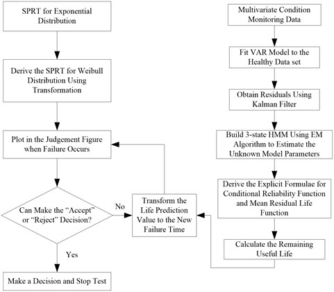
The SPRT plan based on condition monitoring data for Weibull distribution is systematically shown in Fig. 1. To our knowledge, this is the first paper deriving a sequential compliance test plan for Weibull distribution and using condition monitoring data for further decisions. We hope the proposed sequential compliance test plan and the life prediction model can become the standard tool for sequential compliance tests of Weibull distribution, which can accurately carry out fault prediction using condition monitoring data.
The remainder of this paper is organized as follows. In Section 2, we analyze the life distribution of gear historical failure data and derive the sequential test plan for gearbox life distribution based on the standard SPRT for exponential distribution. In Section 3, the healthy portion data of the TSA signals is used to fit a VAR model, and the residuals of the whole data set are obtained. In Section 4, a 3-state HMM for residual process and state process is built. EM algorithm is used to estimate the unknown model parameters, and then the RUL of the operating gearbox is calculated. A comparison with other prediction methods is given. In Section 5, the decision for the gearbox life data is made using SPRT for different methods. Conclusions are presented in Section 6.
2. SPRT for gearbox life distribution
2.1. Gearbox life distribution
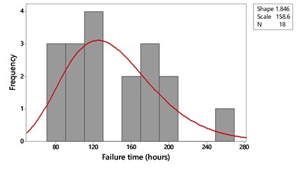
We obtained 18 samples of gearbox life history data for mechanical fault diagnosis from the Applied Research Laboratory at Pennsylvania State University. All the gears worked under the same or similar conditions. A goodness-of-fit test was performed for several probability models to determine the best fitness of the gearbox life data. Four most possible kinds of probability distribution functions were tested, the goodness-of-fit values of which are shown in Fig. 2. It can be seen from Fig. 2 that the life distribution of gears does not obey exponential distribution, therefore the SPRT for the exponential distribution in the standards is not suitable for the gear reliability compliance test. It is shown from the test that the Weibull distribution is the best one for the life of gears with a high -value of 0.450. Its shape and scale parameters are shown in Fig. 3. Next, we derive the sequential compliance testing scheme for Weibull distribution according to the theory of SPRT.
Fig. 2Goodness-of-fit test for gear life data
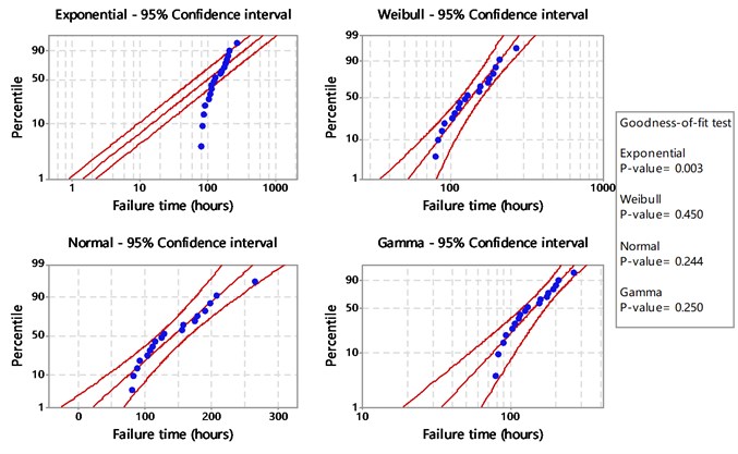
Fig. 3Gear life distribution ft;η,m=m/ηmηm-1e-t/ηm, t≥0, η=158.6, m=1.846
2.2. Operating characteristic curve and sampling risk
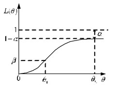
The ideal operating characteristic (OC) curve of sampling is shown in Fig. 4 with as the life expectancy of products. Rules are given that: if the life expectancy of the batch of products , the life of the product is deemed to be qualified, and the acceptance probability ; if not, the life of the product is deemed to be unqualified, and the acceptance probability .
There are two hypotheses existing in the SPRT: : , : , . The sampling test, which determines the whole batch of products through checking the samples, will lead to two types of errors due to the randomness of sampling. A Type I error determines the certified products as uncertified, bringing loss to the producer and rejects when it is true, the probability of which is defined as the producer’s risk . A Type II error determines the uncertified products as certified, bringing loss to the consumer and accepts when it is false, the probability of which is defined as the consumer’s risk . Both the producer and the consumer hope to take lower risk, therefore, the upper test mean time between failure (MTBF) and lower test MTBF are proposed. The acceptance probability changes with ; Fig. 5 displays the actual OC curve of sampling.
Fig. 4The ideal OC curve of sampling
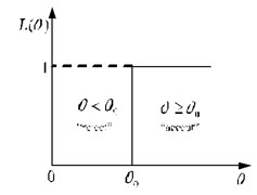
Fig. 5The actual OC curve of sampling
2.3. SPRT for Weibull distribution
The cumulative distribution function (CDF) and probability density function (PDF) of the two-parameter Weibull distribution are given by:
where is shape parameter and is scale parameter.
Assume that the random variable obeys Weibull distribution, the probability distribution function of which is denoted by , where refers to the life parameter. Both producer and consumer take products’ MTBF to verify whether the products meet the reliability requirement or not:
With pre-assigned and , then for the samples , of which the probability density function of population samples are , and the joint probability density function of the random variables is given by:
If , then the joint probability density function is
If , then the joint probability density function is , where is the producer’s risk and is the consumer’s risk.
Then, the probability ratio is . This is the principle of the sequential probability ratio sampling test plan. According to the sequential sampling test rules, two constants, and , need to be chosen. Wald [1] put forward the SPRT judge boundaries: , .
1) If , then , “accept” ( is lager and “accept” with high probability);
2) If , then , “reject” ( is larger and “reject” with high probability);
3) If , then decisions to “accept” or “reject” cannot be made, so the test should be continued.
Judgment criteria for the sequential validation test under the exponential distribution is given in GJB 899A-2009 and MIL-STD-781D [7, 8]. By transforming the two-parameter Weibull distribution into the exponential distribution, the SPRT scheme for Weibull distribution can be obtained. Substituting , into Eq. (1) yields:
Then obeys the exponential distribution, thus the Weibull distribution has been converted to the exponential distribution. Correspondingly, if samples are put into the reliability sequential test and samples fail until with as the failure time of the th sample, then the joint probability density function of the samples is:
The probability that there are failed items before cumulative test time is:
Under the different requirements of MTBF, the probability ratio of failed items before cumulative test time is:
where , .
Different from Hauck and Keats [13], a predetermined reliability must be given when converting to and with Eq. (7), while MTBF is the verification index of product, so the value of will affect the formulation of the test plan.
By substituting and into the Eq. (3), and can be obtained:
The judge boundaries of SPRT is given by:
Taking natural logarithms on both sides of inequality Eq. (10), judge conditions of the SPRT plan for Weibull distribution is given by:
Sequential compliance criterion for Weibull distribution is given by:
where:
is the cumulative failure time, in the non-replacement case:
In the replacement case:
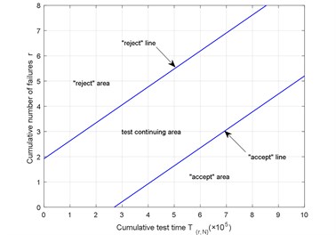
Taking an example of 135, 90, 0.10, 1.846, the sequential schematic diagram for Weibull distribution is shown in Fig. 6. In the sequential test, once the failure occurs, the point should be put into Fig. 6 to make a decision. A point plotted in the “reject” area results in rejecting the hypotheses. A point plotted in the “accept” area results in accepting the hypotheses. Testing continues as long as the point remains in the “test continuing” area.
Fig. 6Schematic of SPRT for Weibull distribution
3. Computation of residuals subject to vibration monitoring
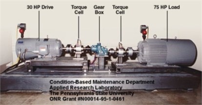
Test data is from the Mechanical Diagnostic Test Bed (MDTB) (Fig. 7) in the Applied Research Laboratory of Condition-Based Maintenance Department at Pennsylvania State University. MDTB is used for gearbox life reliability verification tests of which the indicators are 135, 90 and 0.10.
Fig. 7Mechanical diagnostic test bed
Gearboxes used in this test includes a pinion gear and a drive gear. Four gearboxes with the same specification were tested, of which the test numbers were respectively #5, #10, #12 and #13. #2 and #3 acceleration sensors were installed on the gearbox body, the axial and horizontal direction respectively. The structure diagram of the test scheme is shown in Fig. 8.
The test is divided into two stages: at a constant rotating speed (1750 rpm), gearbox was first run at 100 % output torque for 96 hours (555 in-lbs); then increased to 300 % torque (1665 in-lbs) until failure. Gearbox output torque is shown in Fig. 9 while input shaft speed in Fig. 10. Samples were taken every 30 minutes and stored in a new file with the sampling frequency of 20 kHz. Each sampling time is 10 s. Driving motor speed V01 and gearbox output torque V05 were also collected with sampling frequency of 1 kHz and sampling time of 10 s.
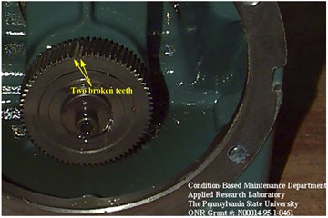
All gearboxes run normally in the first stage, thus vibration signals in the second stage were analyzed. Failure was first found in the #12 gearbox, for which 31 files were collected at 300 % output torque. Files for #2 and #3 sensors were named as A02 and A03, respectively. The original vibration signals are shown in Fig. 11. The results of shutdown fault check presented in Fig. 12 show that the pinion gear was normal while two broken teeth were found in the drive gear without root cracks and midtooth cracks.
Fig. 8Structure diagram of the test scheme
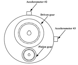
Fig. 9Gearbox output torque V05
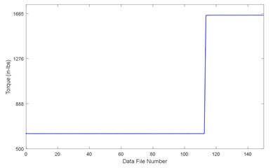
Fig. 10Driving motor input speed V01
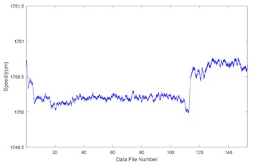
Fig. 11Original data for #12 under 300 % output torque
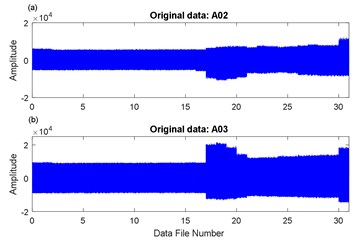
Fig. 12Two broken teeth on drive gear in #12
3.1. Time synchronous averaging (TSA) algorithm
The TSA algorithm is widely applied in fault diagnosis of gears. The TSA signal of vibration monitoring data is given by:
where is the number of sampling points in a single operating period and is the rotation period number included in each sampling data file.
In a complete revolution, the TSA signal of a gear of interest meshing signal in the healthy state is given by:
where is the meshing harmonic number; is the amplitude at the th harmonic frequency (, where is the number of teeth and is the shaft rotation frequency); is the amplitude modulation function, is the initial phase, and is the phase modulation function at the th harmonic.
When a localized fault occurs, the impact-induced resonant vibration in one revolution of the monitored gear is [23]:
where is the envelope function, is the resonance frequency and is the corresponding initial phase. Hence, the measured signal can be written as the following form:
where is the modified amplitude modulation functions at the th harmonic, and is the modified phase modulation functions at the th harmonic.
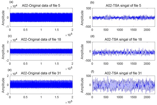
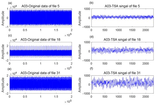
Take for example the #12 gearbox, in which the first failure occurs. File 5, file 18 and file 31 of the data file A02 and A03 at 300 % output torque were selected for TSA signal analysis, which are shown in Fig. 13 and Fig. 14.
Fig. 13A02 data analysis: a) original data of file 5, b) TSA signal of file 5; c) original data of file 18, d) TSA signal of file 18; e) original data of file 31, f) TSA signal of file 31
3.2. Vector autoregression (VAR) model
In this paper, the healthy portion of the TSA signals was used to fit a VAR model. With the established model and estimated model parameters, the residuals of the model can be further calculated. Two-dimensional data can be expressed as , 1, 2. Suppose that the healthy portion of the data obeys a stationary VAR process:
where are independent identically distributed (i.i.d) and follow ; is the autocorrelation matrices; is the mean value; is the covariance; is the model order. Let , Eq. (19) can be transformed as follows:
The Akaike Information Criterion (AIC) criterion is used in this paper to determine the model order , more details can be found in Reinsel [31].
Fig. 14A03 data analysis: a) original data of file 5, b) TSA signal of file 5; c) original data of file 18, d) TSA signal of file 18; e) original data of file 31, f) TSA signal of file 31
3.3. Calculation of residuals
The estimated VAR model parameter can be utilized to calculate the residual of the TSA signals. The residual can be computed as follows:
Taking #12 gearbox as an example, in which failure first occurred. Fig. 15 exhibits the residuals from A02 and A03 data files at 300 % output torque. We selected the root mean square (RMS) of characteristic parameters to process the residuals, which was commonly used in vibration signal processing, to reflect the states of gears, as shown in Fig. 16.
From Fig. 16, the residual RMS values in files 1 to 16 from A02 and A03 sensors are more stable, and we assume this part of the data is the healthy portion. Those in files 17 to 31 increased significantly, therefore we assume this part of the data is the unhealthy portion. Normality and independence tests were carried out for these two parts of data, of which the results are shown in Table 1.
Fig. 15Residuals for data files 1-31
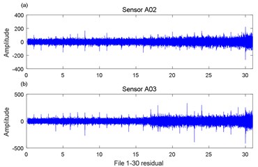
Fig. 16RMS Residuals for data files 1-31
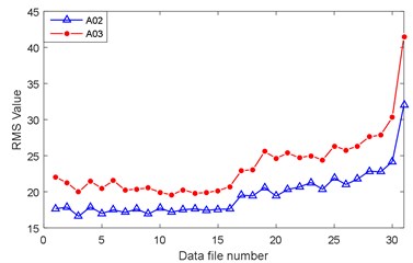
Table 1p-value of the normality and independence tests
RMS of residuals | Healthy portion (files 1-16) | Unhealthy portion (files 17-31) |
Normality (Henze-Zirkler) | 0.1404 | 0.3801 |
Independence (Portmanteau) | 0.2231 | 0.1034 |
From Table 1, both the RMS values of the residuals for A02 and A03 passed the normality and independence tests, indicating that RMS residuals are independent and obey the multivariate normal distribution, which is consistent with the observation values of the HMM in Section 4 follow the multivariate normal distribution.
4. Remaining useful life prediction method based on HMM
4.1. Hidden Markov model (HMM)
Kim et al. [32] showed that a 3-state Markov was sufficient to describe the degradation process. Assume that the gear system can be described by a 3-state HMM (state space is ): state 0 (healthy or good state), state 1 (unhealthy or warning state) and state 2 (failure state). State 0 and state 1 are unobservable. Only state 2 is observable. The system state transition is illustrated in Fig. 17, in which the transition probability matrix is , where denotes the probability that the state transitions from state to state .
Fig. 17Schematic for system state transition of 3-state HMM
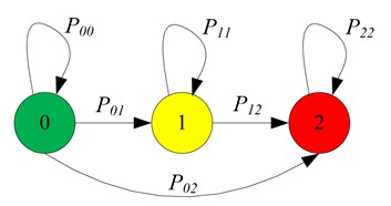
Suppose that the system starts in the healthy state, the instantaneous transition rate matrix is given by:
where , , are unknown parameters.
Let represent the system failure time. Observation is independent given the system state. represents the bivariate observations. Thus, under the condition of state follows a bivariate normal distribution of , 0, 1, and the probability density function is given by:
where , and , are unknown observation parameters.
As the test proceeds, three gearboxes failed in total while the #10 gearbox still worked without failure. The failure times which they shut down for gearboxes #12, #13 and #5 are 111.5 h, 114.5 h and 131 h respectively. With this failure time data, decisions to accept or reject still cannot be made (see Section 5 for analysis results). In fact, three groups of failure data and one group of suspension data provides sufficient information to built a HMM for residual life prediction. Let ,…, denote the failure data sets, where (for #12, #13 and #5 gearboxes). Failure data is expressed by and the respective failure time is , where . Let denote the collected suspension data sets, where (for #10 gearbox). Similarly, suspension data is expressed by and the failure time . represent the observation data and is the corresponding likelihood function, where and are the unknown parameters to be estimated.
The EM algorithm is used to estimate the unknown parameters. The EM algorithm works as follows:
E-step: Compute the pseudo likelihood function:
where and are the initial values; represents the complete data set, in which each failure history and suspension history of the observable data set have been augmented with the unobservable sample path information of the state process.
M-step: Choose , such that:
Updated parameters , in each step are then used as new initial values to the E-step, leading the iteration in E-step and M-step until the Euclidean norm satisfies . The detailed explicit formulae can be found in Kim and Makis [32]. The expectation is updated in each step, for the maximization of which there exists a unique stationary point. The updated explicit formulae for in each step are:
The updated explicit formulae for in each step are:
Initial values are assigned to and and the EM algorithm is used to solve the parameters to be estimated, the convergence criterion of which is . The estimated results are shown in Table 2.
Table 2Model parameters estimation with EM algorithm
Parameters | Initial values | First iteration | Second iteration | Last iteration |
0.5 | 0.0159 | 0.0148 | 0.1515 | |
0.2 | 0.0000 | 0.0000 | 0.0000 | |
0.5 | 0.1042 | 0.2004 | 0.1493 | |
– | –2.02 | –1.94 | –1.87 |
4.2. Remaining useful life prediction
In partially observable Markov decision process (POMDP) theory, is defined as the posterior probability that the system is in the warning state at time given the observations up to time [33]:
According to Bayes’ theorem, at each sampling epoch, the posterior probability can be updated by:
where the initial value . The transition probability matrix , in Eq. (34) can be obtained by solving Kolmogorov backward differential equations, which is given by:
Details can be found in Appendix A.
So, the conditional reliability function of the RUL at sampling point is:
Thus, the PDF of the RUL is:
The MRL is given by:
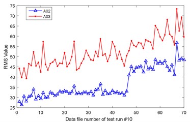
By the time 131 h, 70 data files were collected for #10 gearbox. The original data in A02 and A03 are shown in Fig. 18. In accordance with the data processing method in Section 3, the residuals of RMS values are given in Fig. 19.
Fig. 18Original data of test run #10
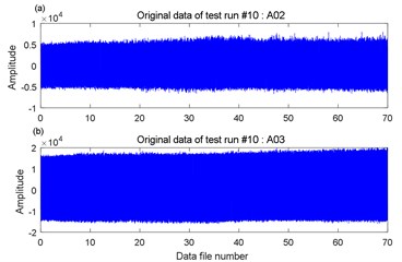
Fig. 19RMS residuals for test run #10
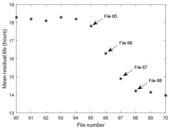
With the estimated model parameters and the observation residuals of sampling files of #10 gearbox, the conditional reliability functions can be updated using the Eq. (36) and the observation values obtained in each sampling. The conditional reliability functions corresponding to files 65 to 70 are shown in Fig. 20. The probability density functions from files 65 to 70 are shown in Fig. 21, where “*” represents the actual residual life. The corresponding mean residual lives are shown in Fig. 22. The predicted RUL is 18.28 hours at file 60. It changes a little up to file 65, meaning that the gearbox operates under a relatively good state. The MRL decreases to 14.13 hours after file 68, which indicates that the gearbox runs in the warning state. It can be found that the actual RUL from file 68 is 14.45 hours, and from file 70 is 13.45 hours, which are very close to the predicted RUL values. Thus, the proposed life prediction approach is applicable to predict the RUL for the gearboxes.
Fig. 20Conditional reliability function
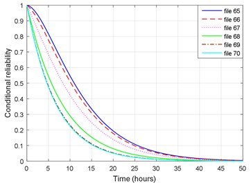
Fig. 21Probability density function
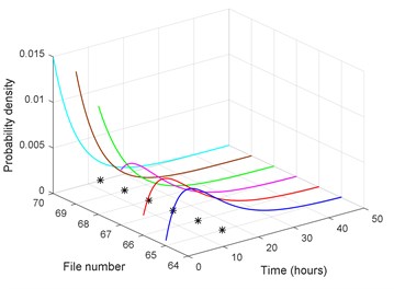
Fig. 22Remaining useful life prediction for #10 gearbox
4.3. Comparison with other prediction methods
In this subsection, the RUL prediction based on HMM is compared with other commonly used prediction methods: (i) stochastic filtering model (SFM) and (ii) Wiener process [26].
In SFM, the unobservable states and the variables related to observable states are used to establish a state space model to describe the degradation process of the system. Suppose that the condition monitoring data in the good and warning states follow the two-parameter Weibull distribution, which is denoted by , where is the scale parameter and is the shape parameter. Therefore, the relationship between and RUL has the following form:
Further, the stochastic relationship between the current condition monitoring data obtained when the gear system starts in the warning state and RUL is given by:
where is the first time when failure occurs.
The unknown model parameters in SFM can be estimated using maximum likelihood estimation (MLE). Thus, the RUL can be further obtained.
Next, the Wiener process is employed to model the deterioration of the gearboxes. Let be the degradation measure at time . In general, the Wiener process can be represented as the following form:
where is the standard Brownian motion, , is the drift parameter, is the diffusion coefficient.
Denoted by is the failure threshold, thus the life of the gear system is defined by the first time that the degradation measure is above the failure threshold, which is given by:
From Eq. (40), the PDF of the RUL can be computed as follows:
Therefore, the expectation of RUL is given by:
The data from files 60 to 70 are selected for MRL prediction. At each sampling epoch, the life prediction is performed when the new observations are available, and then the predicted values using SFM and the Wiener process are compared with that using HMM. Meanwhile, the relative errors (RE) between actual remaining lives (ARL) and the prediction results using different models are calculated, which is given by:
The prediction results are shown in Table 3. Table 3 evidences that with the increased number of collected data, the RE of the prediction results using HMM are smaller than those using SFM and Wiener process, which are closer to the ARL. The average RE using HMM is 3.90 %, while using SFM is 13.60 % and the Wiener process is 7.47 %. Thus, the life prediction method proposed in this paper yields better results than other methods.
Table 3Comparison of RUL prediction and RE using different models
File No. | ARL | RUL | RE | ||||
HMM | SFM | Wiener process | HMM | SFM | Wiener process | ||
60 | 18.45 | 18.28 | 20.34 | 19.50 | 0. 92 | 10.24 | 5.69 |
61 | 17.95 | 18.20 | 20.32 | 19.62 | 1.36 | 12.85 | 9.05 |
62 | 17.45 | 18.09 | 20.18 | 19.21 | 3.47 | 14.80 | 9.54 |
63 | 16.95 | 18.30 | 20.12 | 19.02 | 7.32 | 17.18 | 11.22 |
64 | 16.45 | 18.21 | 20.42 | 18.89 | 9.54 | 21.52 | 13.22 |
65 | 15.95 | 17.82 | 19.63 | 18.5 | 10.14 | 19.95 | 13.82 |
66 | 15.45 | 16.30 | 19.32 | 16.47 | 4.61 | 20.98 | 5.53 |
67 | 14.95 | 14.87 | 16.32 | 15.24 | 0.43 | 7.43 | 1.57 |
68 | 14.45 | 14.13 | 15.71 | 15.02 | 1.73 | 6.83 | 3.09 |
69 | 13.95 | 14.05 | 14.45 | 13.86 | 0.54 | 8.13 | 4.93 |
70 | 13.45 | 13.96 | 12.23 | 12.29 | 2.87 | 9.65 | 4.55 |
5. SPRT of the gearboxes
5.1. SPRT for Weibull distribution
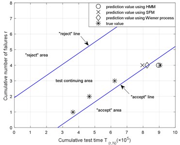
When the gearbox shut down due to failure, the failure time was substituted into the sequential decision diagram and a decision was made. If the failure time point plotted in the “accept” or “reject” area, stop the test and make the decision to “accept” or “reject” the hypotheses; if the point plotted in the “test continuing” area, then no decision will be made and the test needs to be continued until the next failure for further analysis. Fig. 23 exhibits the SPRT decision diagram for Weibull distribution using MRL predictions based on HMM and true life value.
Fig. 23The test judgment figure using Weibull SPRT
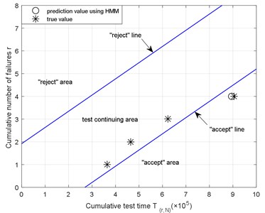
As illustrated in Fig. 23, the life data of the first three gearboxes with failures were put into the SPRT decision diagram for Weibull distribution, finding that three points all plotted in the “test continuing” area, while the life data point of the fourth gearbox plotted in the “accept” area, leading to the “accept” decision. The residual life predicted from the 70th file of the #10 gearbox is 13.96 h, which is very similar to the ARL of 13.45 h. Using the actual failure time of the #10 gearbox, the decision to “accept” is obtained. Thus, the proposed model can be applied to the prediction of the residual life of the gearbox degeneration system.
5.2. Comparison with other compliance methods
We will now compare the proposed SPRT with other reliability sequential compliance methods. It is known that GJB 899A-2009 [7] and MIL-STD-781D [8] provide the standard SPRT for exponential life distribution. Thus, we first consider the exponential SPRT. The four true failure times of the gearboxes and three prediction values of the fourth gearbox were substituted into the exponential SPRT, the results are presented in Fig. 24. As illustrated in Fig. 24, the life data of the first three gearboxes with failure was put into the SPRT decision diagram for exponential distribution. It was found that the first three points all plotted in the “test continuing” area. While the true value and the prediction values that obtained using HMM, SFM and Wiener process all plotted in the “test continuing” area. Neither a decision to “accept” nor “reject” the hypotheses can be made for all four gearboxes using the SPRT for exponential distribution.
We then consider the SPRT decision diagram for Weibull distribution using true values and prediction values. Fig. 25 shows the first three points all plotted in the “test continuing” area, which is similar to the results obtained using exponential SPRT. The fourth life prediction values obtained using SFM and Wiener process all plotted in the “test continuing” area. However, both the prediction value using HMM and the true value plotted in the “accept” area, indicating that the decision to “accept” the hypotheses can be made.
It can be seen from Fig. 24 and Fig. 25 that adopting different life prediction methods and SPRT methods will lead to quite different decisions. In the SPRT for exponential distribution, using the life prediction values and the true values, one can hardly determine whether to accept or reject the hypotheses before all the samples fail. To make further analysis, new samples must be provided for testing. Furthermore, there is no reason to use the SPRT for exponential distribution because the life of the gearboxes in fact obeys Weibull distribution. Better results can be achieved when adopting the SPRT for Weibull distribution using HMM for RUL prediction. We can accept the hypotheses according to the fourth prediction data which is consistent with the results using the ARL value. While based on the life prediction values that used SFM and the Wiener process, neither decision to accept or reject the hypotheses can be made, and the test must continue for further decision making. The comparison shows the efficacy of the prediction method based on HMM and the proposed SPRT for Weibull distribution.
Fig. 24The test judgment figure using exponential SPRT
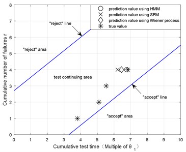
Fig. 25The test judgment figure using Weibull SPRT
6. Conclusions
A novel SPRT method for a partially observable deterioration gear system was proposed in this paper. Specific to the reality that the life of gearboxes obeys the Weibull distribution rather than the exponential distribution, the SPRT method for Weibull distribution was derived, making up for the existing standards, in which the SPRT method only applied to exponential distribution. In order to save test time and reduce the cost, a life prediction model was established using history failure data and existing monitoring data for the life prediction of the operational products. The predicted values were transformed to life failure data used in the SPRT method for Weibull distribution for further decisions. The degradation process of gearboxes was described by a 3-state continuous time HMM. Using the healthy data portion of the TSA signals to build a VAR model, the residuals of the failure data and suspension data were obtained, which were used to estimate the parameters in the HMM with the EM algorithm. The distribution of the RUL and the MRL were calculated and updated with the posterior probability that the system is in the warning state. Meanwhile, the explicit expressions of RUL and MRL were given. We compared the predicted values using HMM with the actual values, which were found to be in agreement with the true values, verifying the validity of the residual life modeling. The life prediction model proposed in this paper was also compared with the methods based on the SFM and Wiener process. The results showed that the HMM was much closer to the actual deterioration process with the smallest RE. The comparison between SPRT for Weibull distribution and the standard SPRT for exponential distribution using different life prediction models further illustrated the limitations of the standard SPRT method, and fake assumptions of the life distributions may lead to undesirable results.
In this paper, we have derived the SPRT method for Weibull distribution and employed the continuous time HMM for life prediction. For future studies, a more general hidden semi-Markov model can be considered, in which the sojourn time for each state obeys the general Erlang distribution, which could be a suitable topic for future research.
References
-
Wald A. Sequential Analysis. Wiley, New York, 1947.
-
Chetouani Y. A sequential probability ratio test (SPRT) to detect changes and process safety monitoring. Process Safety and Environmental Protection, Vol. 92, 2014, p. 206-214.
-
Li D., Chang F. M., Chen K. Building reliability growth model using sequential experiments and the Bayesian theorem for small datasets. Expert Systems with Applications, Vol. 37, 2010, p. 3434-3443.
-
Kira S., Yang T., Shadlen M. N. A neural implementation of Wald’s sequential probability ratio test. Neuron, Vol. 85, 2015, p. 861-873.
-
Ou Y., Wu Z., Chen S., Lee K. M. An improved SPRT control chart for monitoring process mean. The International Journal of Advanced Manufacturing Technology, Vol. 51, 2010, p. 1045-1054.
-
Ou Y., Wu Z., Yu F., Shamsuzzaman M. An SPRT control chart with variable sampling intervals. The International Journal of Advanced Manufacturing Technology, Vol. 56, 2011, p. 1149-1158.
-
Reliability Testing for Qualification and Production Acceptance. Technical Report GJB 899A-2009, China, 2009.
-
Military Standard Reliability Testing for Engineering Development, Qualification, and Production. Technical Report MIL-STD-781D, USA, 1986.
-
Guo B., Jiang P., Xing Y. Y. A censored sequential posterior odd test (SPOT) method for verification of the mean time to repair. IEEE Transactions on Reliability, Vol. 57, 2008, p. 243-247.
-
Nelson W. Accelerated Testing: Statistical Models, Test Plans, and Data Analyses. Wiley, New York, 1990.
-
Rolling Bearings-Test and Assessment for Life and Reliability. Technical Report GB/T 24607-2009, China, 2009.
-
An Z. W., Zhang Y., Liu B. A method to determine the life distribution function of components for wind turbine gearbox. Journal of University of Electronic Science and Technology of China, Vol. 43, 2014, p. 950-953.
-
Hauck D. J., Keats J. B. Robustness of the exponential sequential probability ratio test (SPRT) when Weibull distributed failures are transformed using a “known” shape parameter. Microelectronics Reliability, Vol. 37, 1997, p. 1835-1840.
-
Tsai T., Lu Y., Wu S. Reliability sampling plans for Weibull distribution with limited capacity of test facility. Computers and Industrial Engineering, Vol. 55, 2008, p. 721-728.
-
Pandit P. V., Gudaganavar N. V. On robustness of a sequential test for scale parameter of Gamma and exponential distributions. Applied Mathematics, Vol. 1, 2010, p. 274-278.
-
Deng Q., Yuan H. J. Sequential compliance test method for lognormal distribution. Journal of Beijing University of Aeronautics and Astronautics, Vol. 38, 2012, p. 1-4.
-
Li X., Cai J., Zuo H. F., et. al. Research on reliability sequential compliance method for rolling bearings. Journal of Information and Computational Science, Vol. 12, 2015, p. 5309-5318.
-
Li Y. B., Xu M. Q., Wei Y., Huang W. H. An improvement EMD method based on the optimized rational Hermite interpolation approach and its application to gear fault diagnosis. Measurement, Vol. 63, 2015, p. 330-345.
-
Li Y. B., Xu M. Q., Wei Y., Huang W. H. Health condition monitoring and early fault diagnosis of bearings using SDF and intrinsic characteristic-scale decomposition. IEEE Transactions on Instrumentation and Measurement, Vol. 65, Issue 9, 2016, p. 2174-2189.
-
Igba J., Alemzadeh K., Durugbo C., Henningsen K. Performance assessment of wind turbine gearboxes using in-service data: current approaches and future trends. Renewable and Sustainable Energy Reviews, Vol. 50, 2015, p. 144-159.
-
Braun S. The synchronous (time domain) average revisited. Mechanical Systems and Signal Processing, Vol. 25, 2011, p. 1087-1102.
-
Wang X., Makis V. Autoregressive model-based gear shaft fault diagnosis using the Kolmogorov-Smirnov test. Journal of Sound and Vibration, Vol. 327, 2009, p. 413-423.
-
Wang W. Y., Wong A. K. Autoregressive model-based gear fault diagnosis. Journal of Vibration and Acoustics-Transactions of the ASME, Vol. 124, 2002, p. 172-179.
-
Gales M., Young S. The application of hidden Markov models in speech recognition. Foundations and Trends in Signal Processing, Vol. 1, 2007, p. 195-304.
-
Lu C., Li T. Y., Liu H. M. Online milling tool condition monitoring with a single continuous hidden Markov models approach. Journal of Vibroengineering, Vol. 16, Issue 5, 2014, p. 2448-2457.
-
Si X., Wang W., Hu C. Remaining useful life estimation – a review on the statistical data driven approaches. European Journal of Operational Research, Vol. 213, Issue 1, 2011, p. 1-14.
-
Jiang R., Yu J., Makis V. Optimal Bayesian estimation and control scheme for gear shaft fault detection. Computers and Industrial Engineering, Vol. 63, 2012, p. 754-762.
-
Kim M. J., Makis V., Jiang R. Parameter estimation in a condition-based maintenance model. Statistics and Probability Letters, Vol. 80, 2010, p. 1633-1639.
-
Kim M. J., Jiang R., Makis V., Lee C. Optimal Bayesian fault prediction scheme for a partially observable system subject to random failure. European Journal of Operational Research, Vol. 214, 2011, p. 331-339.
-
Peng Y., Dong M., Zuo M. J. Current status of machine prognostics in condition-based maintenance: a review. The International Journal of Advanced Manufacturing Technology, Vol. 50, 2010, p. 297-313.
-
Reinsel G. C. Elements of Multivariate Time Series Analysis. Springer, New York, 1997.
-
Kim M. J., Makis V., Jiang R. Parameter estimation for partially observable systems subject to random failure. Applied Stochastic Models in Business and Industry, Vol. 29, 2013, p. 279-294.
-
Makis V. Multivariate Bayesian control chart. Operations Research, Vol. 56, Issue 2, 2008, p. 487-496.
About this article
The authors are grateful to Prof. Viliam Makis from the University of Toronto. This Research was co-supported by the Fundamental Research Funds for the Central Universities (No. NS2015072) and the Funding of Jiangsu Innovation Program for Graduate Education (KYLX15_0313). Also, the support provided by China Scholarship Council (CSC) during a visit of Xin Li at the University of Toronto is acknowledged and appreciated.
Xin Li contributed to the data analysis and manuscript preparation. Jing Cai approved the final version. Hongfu Zuo contributed to the conception of the study. Xi Chen performed the derivation of the reliability sequential method. Huijie Mao helped perform the comparison. Yutong Xu helped perform the analysis with constructive discussions.
