Engine remaining useful life prediction based on trajectory similarity

Liu, Xin; Jia, Yunxian; Zhou, Jie; Liu, Tianbin

Vibroengineering Procedia

Browse Procedia

Published: 08 December 2016

Check for updates

Engine remaining useful life prediction based on trajectory similarity

Xin Liu¹

Yunxian Jia²

Jie Zhou³

Tianbin Liu⁴

^{1, 2, 3}Department of Equipment Command and Management. Ordnance Engineering College, Shijiazhuang, China

⁴94270 Unit, PLA, Jinan, China

Corresponding Author:

Xin Liu

Cite the article Download PDF

Downloads 1517

Abstract

The traditional remaining useful life prediction methods need to study the mechanism failure of equipment and the vibration signals can easily be submerged by the noise in the actual operation, in order to solve these problems, the methods of Trajectory similarity based prediction (TSBP) and condition monitoring based on lubricant information are proposed in this paper. The gradient model of lubricant data information which is processed by principal component analysis (PCA) is used to monitor equipment status. Additionally, degradation trajectory abstraction procedure and similarity evaluation procedure are studied in detail. Finally, the both studies are combined for the research of engine remaining useful life prediction and case study proves the simplicity and effectiveness of this method.

1. Introduction

With the increase of the weaponry function, the structure of equipment is more complex correspondingly. To ensure the normal training, a higher requirement for maintenance and support is proposed for the whole life cycle of the equipment. As the key factor of Condition based maintenance (CBM), remaining useful life prediction has an important practical significance for maintenance decision, reducing maintenance and support costs, and improving equipment reliability [1, 2]. The method of trajectory similarity based prediction can directly use historical data to predict the remaining useful life and the degradation mechanism modeling is not required, making it suitable for predicting the remaining useful life of complex equipment.

The vibration signals are often used for the equipment status monitoring, particularly mechanical systems. Due to the complexity of the equipment itself and its working environment with noise, the vibration information can not accurately reflect the equipment status. Therefore, taking use of lubricant data monitoring equipment status can avoid this case effectively [3]. The method of remaining useful life prediction based on lubricant data and trajectory similarity is proposed by combining the advantages of trajectory similarity based prediction and equipment condition monitoring carried out by the lubricant data. Then the method is applied to the remaining useful life prediction of an engine and the case study is used to verify its effectiveness.

2. The method of lubricant data analysis

2.1. Lubricant data model

Currently, the spectrometric lubricant data analysis is the most important technique to get the best lubricant data analysis result. Spectrometric lubricant data analysis is used to analyze the composition and content of metals in lubricating with atomic absorption or atomic emission spectroscopy, in order to determine the failure parts and the degree of damage. Spectrometric lubricant data analysis is not only qualitative judgment of failure parts, but also determined the degree of damage by analyzing how much wear metal component content in the lubricant [4]. By an optical spectrum analyzer for the lubricant under different types of equipment run time analysis, spectral analysis will get a series of data, which contains a large amount of current equipment status information.

To describe the relationship between the lubricant data and equipment status, lubricant concentration analysis model, gradient analysis model and ratio analysis model are the commonly used models. Since the presence of lubricant changes and other operations in the monitoring process, which will lead to a greater impact for the concentration of lubricant, the states estimation of the equipment will be affected. Therefore, we need lubricant data preprocessing to reduce this effect. The density gradient analysis model and ratio analysis model will bring a smaller proportion of affected. In this case, we use density gradient information analysis model to make a correct assessment and the state prediction of degradation equipment.

2.2. Lubricant data preprocessing

The purpose of data preprocessing is making original data suit the trajectory similarity based prediction. In this paper, principal component analysis is used for data preprocessing. Principal component analysis is a method which uses linear conversion to make the original variable to become a list of unrelated variables, which are called principal components. The method can effectively reduce the dimension of the original data, which can be used to simplify the original data. Since the principal component analysis is a basal mathematical analysis method, the method will not be discussed in this paper in detail. This method is applied directly to the lubricant data preprocessing.

In this paper, the data is derived from the literature [5]. A total of four engines are taken as the subject in the experiment. These engines operate in essentially the same condition, with a load of about 300 N·m, and lubricant sample collection is basically 40 hours once. Sample 1, 3 and 4 are used for degradation trajectory abstraction and similarity evaluation, as well as, sample 2 is used for prediction. Through the analysis of friction pair in the engine, the key consideration in the lubricant spectrum are 8 kinds of element, for Fe, Al, Pb, B, Ba, Gr, Mg, and Si.

3. Trajectory similarity based prediction

The main idea of trajectory similarity based prediction is this: If the degradation trajectory of the equipment which is predicted is tracked with the degradation trajectory of equipment which the whole life history is known at a certain time [ $t_{1}$ , $t_{2}$ ], we consider that the two equipments have the similar remaining useful life at the certain time [ $t_{1}$ , $t_{2}$ ]. The equipment which is predicted is called service equipment, and the equipment which historical degradation process is known is called reference equipment.

Fig. 1General procedures of TSBP approach for RUL estimation

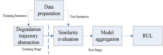
The based framework of trajectory similarity based prediction includes degradation feature extraction, degradation trajectory abstraction, similarity evaluation and remaining useful life prediction [6]. Trajectory similarity based prediction can provide predictive modeling results without modeling the degradation signal of the components, while most other methods are required for modeling the degradation, in the case of non-linear recession, recession modeling is sometimes difficult, which highlights the superiority of the method trajectory similarity based prediction. In the same way, we can get the results of feature dimension reduction for sample 1, sample 3 and sample 4, which will be used in remaining useful life prediction. The general procedures of trajectory similarity based prediction for RUL estimation is shown in Fig. 1.

Degradation trajectory abstraction and similarity evaluation are the key of trajectory similarity based prediction. The exponential curve fitting, moving average filter and interpolation, kernel regression smoothing and relevance vector machines are the common way to make the degradation trajectory [7, 8]. Through a comprehensive analysis, we take kernel regression smoothing as the way to achieve the degradation trajectory. It does not require prior assumptions the form of a function before starting to calculate the complex equipment status at the unknown time, which makes it has a strong adaptability [9].

The expression of kernel function normally:

1

z (t) = \frac{\sum_{i = 1}^{E} K (t, t_{i}) z_{i}}{\sum_{i = 1}^{E} k (t, t_{i})},

where $K ()$ is the Kernel function. In most cases, the Gaussian kernel is used:

2

K_{G} (x, y) = e x p (- \frac{{‖x - y‖}^{2}}{2 ρ^{2}}),

where $ρ$ is the kernel width, a free parameter that has to be specified based on the data, usually through cross-validation.

After selecting the degradation trajectory abstraction method, degradation trajectory function is needed to calculate the similarity of reference equipment and service equipment. In this paper, the minimum Euclidean distance is selected to calculate the similarity.

In the minimum Euclidean distance, the square of the distance between reference equipment $G$ and service equipment $z$ is expressed as:

3

D^{2} = \frac{1}{L} \sum_{i = 1}^{L} {‖z_{i} - g (t_{i})‖}^{2} .

The $M$ variables in $z$ are independent which follow the normal distribution $σ_{m}^{2}$ ( $m =$ 1, 2,…, $M$ ) for each variable respectively, then the likelihood function of $G$ for $z$ is as follow:

4

L (Z | G) = \prod_{i = 1}^{L} \prod_{m = 1}^{M} ({(2 π σ_{m}^{2})}^{- 1 / 2} e x p (- \frac{{(z_{m i} - g_{m} (t_{i}))}^{2}}{2 σ_{m}^{2}}))

= {(\prod_{m = 1}^{M} ({(2 π σ_{m}^{2})}^{- 1 / 2}))}^{L} e x p (- \sum_{i = 1}^{L} \sum_{m = 1}^{M} \frac{{(z_{m i} - g_{m} (t_{i}))}^{2}}{2 σ_{m}^{2}})

= {(\prod_{m = 1}^{M} {(2 π σ_{m}^{2})}^{- 1 / 2} e x p (- \frac{1}{L} \sum_{i = 1}^{L} \sum_{m = 1}^{M} \frac{{(z_{m i} - g_{m} (t_{i}))}^{2}}{2 σ_{m}^{2}}))}^{L} .

Defined similarity $S$ to $L$ th root of the likelihood function $L (Z | G)$ :

5

S = {(L (Z | G))}^{\frac{1}{L}} = \prod_{m = 1}^{M} {(2 π σ_{m}^{2})}^{- 1 / 2} e x p (- \frac{1}{L} \sum_{i = 1}^{L} \sum_{m = 1}^{M} \frac{{(z_{m i} - g_{m} (t_{i}))}^{2}}{2 σ_{m}^{2}}) .

Because $\prod_{m = 1}^{M} {(2 π σ_{m}^{2})}^{- 1 / 2}$ is a constant, so $S$ is simplified:

6

S = e x p (- \frac{1}{L} \sum_{i = 1}^{L} \sum_{m = 1}^{M} \frac{{(z_{m i} - g_{m} (t_{i}))}^{2}}{2 σ_{m}^{2}}),

7

D^{2} = - l n S = \frac{1}{L} \sum_{i = 1}^{L} \sum_{m = 1}^{M} \frac{{(z_{m i} - g_{m} (t_{i}))}^{2}}{2 σ_{m}^{2}}, 0 \leq t \leq t_{E} .

In this case, we need to look for the most delay $τ$ to take the minimum Euclidean distance in that time period:

8

D^{2} = \underset{τ}{m i n} d^{2} (Z, G, τ),

9

d^{2} (Z, G, τ) = \frac{1}{L} \sum_{i = 1}^{L} \sum_{m = 1}^{M} \frac{{(z_{m i} - g_{m} (t_{i} + τ))}^{2}}{2 σ_{m}^{2}},

where $t_{i}$ is in the time point corresponding to $z_{i}$ , and $- τ \leq t_{i} \leq t_{E} - τ$ .

Therefore, to compare the similarity of reference equipment and service equipment at the same time, which find the minimum Euclidean distance between the two equipments by moving the axis, and the minimum value is used to evaluate the similarity between the two equipments.

4. Case studies

The original data sample 1, 3 and 4 is considered as the historical samples, and we will predict the remaining useful life of sample 2, which gradient value is processed by the principal component analysis, taking sample 1 as an example to obtain the correlation matrix $A$ via SPSS:

10

A = \frac{Z^{T} Z}{n - 1} = [\begin{matrix} 1.000 & - 0.565 & - 0.328 & - 0.802 & - 0.116 & - 0.694 & 0.328 & - 0.058 \\ - 0.565 & 1.000 & 0.774 & 0.856 & - 0.148 & 0.878 & - 0.545 & - 0.061 \\ - 0.328 & 0.774 & 1.000 & 0.812 & 0.371 & 0.889 & 0.013 & - 0.048 \\ - 0.802 & 0.856 & 0.812 & 1.000 & 0.257 & 0.984 & - 0.248 & 0.009 \\ - 0.116 & - 0.148 & 0.371 & 0.257 & 1.000 & 0.265 & 0.803 & 0.175 \\ - 0.694 & 0.878 & 0.889 & 0.984 & 0.265 & 1.000 & - 0.222 & - 0.007 \\ 0.328 & - 0.545 & 0.013 & - 0.248 & 0.803 & - 0.222 & 1.000 & 0.049 \\ - 0.058 & - 0.061 & - 0.048 & 0.009 & 0.175 & - 0.007 & 0.049 & 1.000 \end{matrix}],

where $Z$ is the standardization of the original data matrix $X$ .

Factors are extracted in the order, the eigenvalue of the factor which change with the number of factors is call scree plot, and we can get the load diagram as well. As shown in Fig. 2.

Fig. 2a) The Scree plot and b) load diagram of the principal component analysis

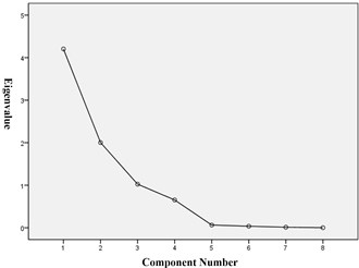
a)

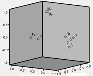
b)

According to the principle of selecting a principal component factor, the first three factors are selected, which eigenvalue is more than 1, and the cumulative variance was 90.404 %, so the first three factors can be more complete description of the original data characteristics.

Finally, to obtain principal components:

11

U = X B,

where $B$ is a component matrix, and we can get the principal component analysis results of sample 1 by calculating, as shown in Table 1.

Similarly, we can get the feature reduction results of sample 3 and sample 4, which will be applied in trajectory similarity based prediction.

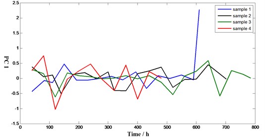
As we can see in Fig. 3, principle component curves are obtained by minimum Euclidean distance which can describe the similarity of all samples. For example, Similarity between sample 2 and other samples with RULs at time 200 are shown in Table 2, which can be used for predict the remaining useful life.

Table 1The principal component analysis results of sample 1

Time ( $t$ )	Independent component 1	Independent component 2	Independent component 3
40	–0.43211	0.135593	–0.05631
82	–0.07654	–0.15747	–0.5858
110	–0.14437	0.014916	–0.17324
150	0.468536	–0.12436	0.286589
192	–0.05698	–0.0673	–0.35019
230	–0.06388	0.014515	–0.0515
272	–0.00918	0.073744	–0.01222
311.3	0.057271	–0.12686	0.010509
350	–0.04957	0.114443	–0.04884
394	0.206628	–0.09029	0.088869
430	–0.33129	0.750251	–0.10646
470	0.082231	–0.56947	0.028855
510	–0.0083	–0.03168	0.003467
550	0.11019	0.01819	0.013007
590	–0.05113	–0.03623	0.021006
610	2.276061	–0.13869	0.357267

Fig. 3First principle component curves of samples

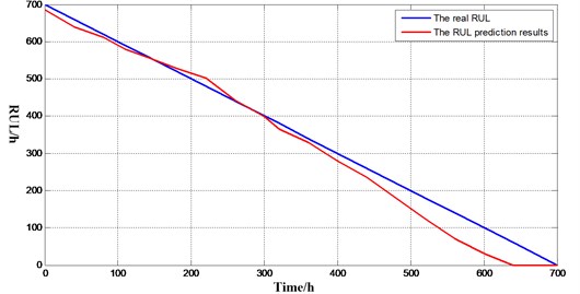
The results of engine remaining useful life prediction based on lubricant data and trajectory similarity is shown in Fig. 4. As we can see, in the early stage, since each of the equipments is in normal condition, the prediction results are decided by the real life of integrated equipments which is an average estimate of remaining useful life, so it does not fit the actual remaining useful life well. Then run to the middle of the life, remaining useful life prediction and the actual operating results are close. When equipments run into the end of its life, a serious deviation is happened. The reference sample is too small and most of the reference sample life is less than the life of the service equipment, resulting in a life expectancy less than the actual life, so we can’t get the strict result in this case. This method has limitations when the sample is small.

Table 2Similarity between sample 2 and other samples with RULs (T= 200 h)

No.	1	3	4
Similarity	0.72	0.83	0.67
RUL	410	585	282

Fig. 4The result of RUL

5. Conclusions

Trajectory similarity based prediction is a newly emerging method, which is used for engine remaining life prediction in this paper. The methods of monitoring the equipment state based on lubricant data and the key step of remaining useful life prediction based on similarity are introduced. Through the case study, the advantage of the method is very obvious, which does not require analysis the failure mechanisms of equipment, at the same time, exposed the shortcoming that requires large raw data. The case study shows that the method for predicting the remaining useful life of complex equipment has the advantages of high accuracy and simplicity.

References

Ren Guoquan, Zheng Haiqi, Zhang Yingtang, et al. A study on the monitoring of wearing conditions in engines based on oil analysis. Acta Armamentarii, Vol. 23, Issue 2, 2002, p. 26-29.

Search CrossRef
Liu Chang Study on Remaining Useful Life Prediction Method of Complex Equipment Life Based on Similarity. Ordnance Engineering College, Shijiazhuang, 2014.

Search CrossRef
Sun Lei, Jia Yunxian, Cai Liying, et al. Research on engine remaining useful life prediction based on oil spectrum analysis and particle filtering. Spectroscopy and Spectral Analysis, Vol. 33, Issue 9, 2013, p. 2478-2482.

Search CrossRef
Zhang Yingbo, Jia Yunxian, Qiu Guodong, et al. Stochastic filtering residual useful life prediction model based on metal concentration gradient in lubricant. Systems Engineering – Theory and Practice, Vol. 34, Issue 6, 2014, p. 1620-1625.

Search CrossRef
Chen Li Condition Based Maintenance Model and Application. Ordnance Engineering College, Shijiazhuang, 2008.

Search CrossRef
Liu Chang, Meng Chen, Wang Cheng Data prediction of RUL prediction based on similarity. Computer and Digital Engineering, Vol. 43, Issue 6, 2015, p. 1009-1013.

Search CrossRef
You Mingyi Robustness and Uncertainty of a similarity-based component remaining life prediction. Electronic Product Reliability and Environmental Testing, Vol. 29, Issue 6, 2011, p. 10-18.

Search CrossRef
Lei Congying, Xia Lianghua, Lin Zhisong Research on similarity-based remaining life prediction of equipment components. Fire Control and Command Control, Vol. 39, Issue 4, 2014, p. 91-94.

Search CrossRef
Wang Tianyi Trajectory Similarity Based Prediction for Remaining Useful Life Estimation. University of Cincinnati, 2010.

Search CrossRef

About this article

Received

13 September 2016

Accepted

19 September 2016

Published

08 December 2016

SUBJECTS

Fault diagnosis based on vibration signal analysis

Keywords

gradient feature

principal component analysis

trajectory similarity based prediction

similarity evaluation

engine

This is an open access article distributed under the Creative Commons Attribution License, which permits unrestricted use, distribution, and reproduction in any medium, provided the original work is properly cited.