Nonlinear factor analysis and its application to acoustical source separation and identification

2.1. Nonlinear Factor Analysis Model

Considering a physical system of $m$ observations $\mathbf{X}\left(t\right)={\left[{\mathbf{x}}_1\left(t\right),{\mathbf{x}}_2\left(t\right),\cdots ,{\mathbf{x}}_m\left(t\right)\right]}^T$, $n$ sources $\mathbf{S}\left(t\right)={\left[{\mathbf{s}}_1\left(t\right),{\mathbf{s}}_2\left(t\right),\cdots ,{\mathbf{s}}_n\left(t\right)\right]}^T$, and noises $\mathbf{N}\left(t\right)={\left[{\mathbf{n}}_1\left(t\right),{\mathbf{n}}_2\left(t\right),\cdots ,{\mathbf{n}}_m\left(t\right)\right]}^T$. The mixing mode of all the sources can be expressed as a function $f\left(\right)$ as a parametrised mapping from source space to observation space, which is shown in Fig. 1. Thus nonlinear factor analysis can be modeled about how the observations are generated from the sources [31]:

If noises can be ignored or treated as sources, the above model can be further simplified as:

Fig. 1The mapping from sources to observations by MLP network

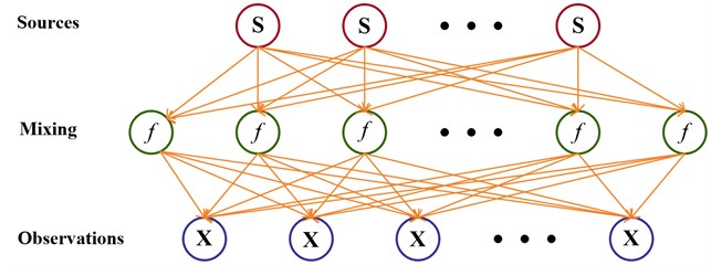
In Fig. 1, the nonlinearity of each hidden neuron is the hyperbolic tangent, which is the same as the usual logistic sigmoid except for a scaling. The mapping can be defined as:

where matrices $\mathbf{A}$ and $\mathbf{B}$ are weights of first and second layer, $a$ and $b$ are corresponding biases.

The sources are assumed to have zero mean Gaussian distributions and again the variances are parametrised by log-std ${\mathbf{v}}_s$, and the noise is assumed to be independent and Gaussian. Therefore, all the parameters are considered to have following distributions:

The prior distributions of $m_a$, ${\mathbf{v}}_a$, $m_b$, ${\mathbf{v}}_b$, the six hyper-parameters $m_{{\mathbf{v}}_{\mathbf{s}}}$,…, $m_{{\mathbf{v}}_B}$ are assumed to be Gaussian with zero mean and standard deviation, and the priors are assumed to be very flat.

2.2. Objective function

If there are only the observations $\mathbf{X}$, the posterior pdf of all the hidden sources should be approximated. Thus the objective function measures the misfit between the actual posterior pdf $p\left(\mathbf{S}\left|\mathbf{X}\right.\right)$ and its approximation $q\left(\mathbf{S}\left|\mathbf{X}\right.\right)$:

Each individual approximation $q\left({\mathbf{s}}_i\left|\mathbf{X}\right.\right)$ is parametrised by the posterior mean ${\stackrel{-}{\mathbf{s}}}_i$ and variance ${\tilde{\mathbf{s}}}_i$ of the parameter. The objective function $C_{\mathbf{S}}(\mathbf{X};\stackrel{-}{\mathbf{S}};\tilde{\mathbf{S}})$ contains $C_q(\mathbf{X};\mathbf{S})$ and $C_p(\mathbf{X};\mathbf{S})$:

Since $\mathbf{S}$, $m_{\mathbf{S}}$, ${\mathbf{V}}_{\mathbf{S}}$ are independent in $q$, the expectation over $q$ produces:

From Eq. (4), there has:

where $\tilde{f}\left({\mathbf{x}}_i\right)$ denotes the total posterior variance of the output $f\left({\mathbf{x}}_i\right)$, and ${\tilde{f}}^{\mathrm{*}}\left({\mathbf{x}}_i\right)$ denotes the variance originating from the weights and biases.

2.3. Parameter updating rules

After the objective function is constructed, the next step is using optimization algorithm to minimize the $C_{\mathbf{S}}(\mathbf{X};\stackrel{-}{\mathbf{S}},\tilde{\mathbf{S}})$ with respect to the posterior means $\stackrel{-}{\mathbf{S}}$ and variances $\tilde{\mathbf{S}}$ of the unknown variables. The fixed point equation is used to update the variances:

Newton iteration is used as posterior variances $\tilde{\mathbf{S}}$ containing the information about the second order derivatives of the objective function $C_{\mathbf{S}}(\mathbf{X};\stackrel{-}{\mathbf{S}},\mathrm{}\tilde{\mathbf{S}})$, and there has:

where ${\alpha }_{\stackrel{-}{\mathbf{s}}}$ is a learning parameter to dampen the oscillations in the fixed point algorithms according to the following rule:

2.4. Source Identification

As some information of sources for mechanical systems normally can be obtained by the theory studies or Instructions, a waveform correlation is constructed to identify the source information by the correlation analysis between the sources and the separated signals. For discrete signals $\mathbf{s}\left(t\right)$ and $\mathbf{y}\left(t\right)$, the waveform correlation coefficient ${\rho }_W$ is defined as:

where:

and $T$ is the data length.

3.1. Introductions

In this section, typical signals of mechanical systems are artificially generated, which are used to test the effects by numbers of hidden neurons and mixed signals on the separation performances of NLFA. Since acoustical signals transmit from sources to measured points mainly through air, and the generating mechanisms of sources are statistically different. Therefore, all the sources are considered to be linearly mixed and independent from each other.

Source signals are: signal ${\mathbf{s}}_1\left(t\right)$ is a periodic wave of oscillating attenuation that simulates mechanical shocks; signal ${\mathbf{s}}_2\left(t\right)$ is a sinusoidal wave that simulates a vibration signal of rotational equipment; signal ${\mathbf{s}}_3\left(t\right)$ is a periodic wave that simulates amplitude modulation; signal ${\mathbf{s}}_4\left(t\right)$ is a white noise that simulates environmental noises. In the numerical case study, the noise is considered to be one source, and the generating functions of the sources are listed as follows:

where $u\left(t\right)$ is a step function.

Generally, the measured signals are mixed signals of all the sources. Therefore, linear superposition is applied to artificially produce the mixed signals, and the mixing matrix $\mathbf{A}$ is randomly generated as shown in the following matrix:

The waveforms of source signals and mixed signals are shown in Fig. 2 and Fig. 3, respectively. Obviously, from Fig. 2 it can be seen that all the source signals have typical wave features. However, from Fig. 3 it is very difficult to identify the features of the sources as all the waveforms of sources are coupling together. Therefore, nonlinear factor analysis is applied to separate the mixed signals into uncorrelated factors, and then source identification can be carried out by a correlation analysis between the separated factors and the given sources.

Fig. 2Waveforms of source signals

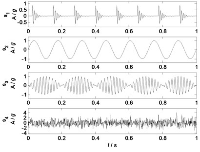
Fig. 3Waveforms of mixed signals

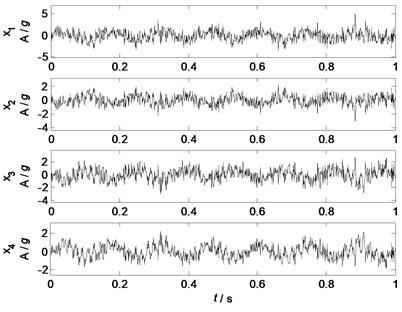
Fig. 4Separated factor 1 by NLFA

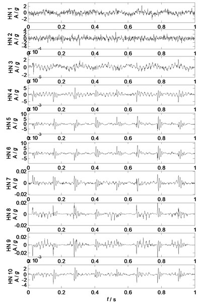
Fig. 5Separated factor 2 by NLFA

3.2. Effects by numbers of hidden neurons

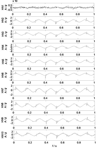
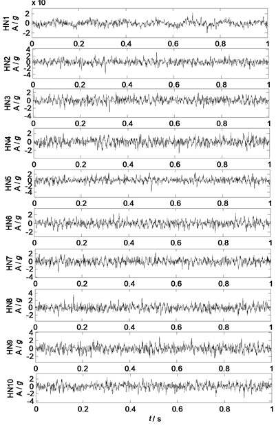
To test the effects by numbers of hidden neurons (HN), four mixed signals are separated into four separated factors using nonlinear factor analysis with different numbers of hidden neurons, and the waveforms of each separated component in different separating conditions are shown in Fig. 4-7.

Fig. 4-7 show the waveforms of different separated factors by NLFA with different HN: Fig. 4 shows that the major feature of source 1 can be extracted as HN is no less than 4, Fig. 5 shows that the major features of source 2 are extracted as HN is no less than 2, Fig. 6 shows that the major features of source 3 can be extracted as HN is no less than 3, and Fig. 7 shows that the major feature of source 4 can be extracted as HN is no less than 2. Generally, the separation performances of NLFA become better as the number of HN increases (HN $<$ 4), and then the separation performances change very little as HN increases (HN $\ge$ 4).

Fig. 6Separated factor 3 by NLFA

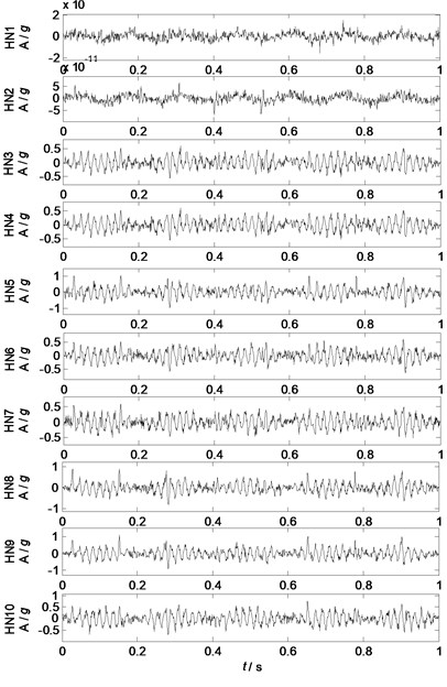
Fig. 7Separated factor 4 by NLFA

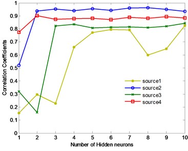
The waveform correlation coefficients between the separated components and related sources are shown in Fig. 8: the separation performances become better as the number of HN increases (HN$\le \mathrm{}$5), and change very litter (HN $>$ 5), the source 2 and source 4 can be well separated as HN is only 2. Generally, increasing the number of HN can improve the separation performances, but it also costs more calculating time (Cost time: 15.44 s (HN2), 16.09 s (HN3), 16.35 s (HN4), 17.25 s (HN5), 17.70 s (HN6), 18.22 s (HN7), 19.60 s (HN8), 21.90 s (HN9), 22.26 s (HN10)). Moreover, as the number of HN increases, there also can cost calculating errors which can be found at the curve of separated factor 1 in Fig. 8. Therefore, normally the number of HN should be as less as possible to improve the calculating efficiency and avoid additional calculating errors. From Fig. 8, the number of HN is suggested to be 5-7.

Fig. 8Waveform correlation coefficients

3.3. Effects by numbers of mixed signals

To test the effects by numbers of mixed signals, the number $m$ of mixed signals are set from 2 to 10, and each mixed signals are generated by all the sources with a randomly mixing matrix. Then the mixed signals are separated by NLFA, and the waveforms of separated components in different conditions are shown in Fig. 9-12.

Fig. 9Separated components (m= 2)

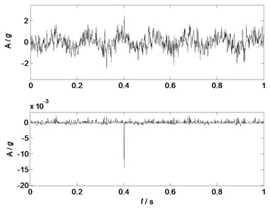
Fig. 10Separated components 4 (m= 3)

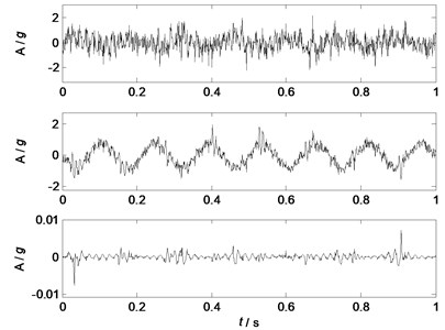
Fig. 11Separated components (m= 4)

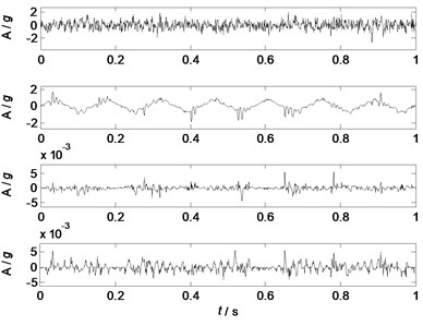
Fig. 12Separated components (m= 5)

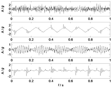
Fig. 9-12 show the waveforms of separated factors as the numbers of the mixed signals are 2, 3, 4 and 5 respectively. Fig. 9 ($m=$ 2) shows that 2 factors are separated from two mixed signals, and only a noisy sine wave but no other source feature is separated. Fig. 10 ($m=$ 3) shows that 3 components are separated from 3 mixed signals, and only the sine wave are well separated. Fig. 11 shows that 4 components are separated from 4 mixed signals, and the major features of source 2 and source 4 are well separated. The features of source 1 and source 3 are separated, but the features are not clear as they are still coupling with other waveforms. Fig. 12 shows that 4 components are separated from 5 mixed signals, and the major features of all the sources are well separated. Therefore, in this case study, the separation performances of NLFA become better as the number of the mixed signals increases.

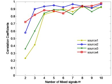
To quantitatively reveals effects by the number of the mixed signals, more numerical case studies are provided, and correlation coefficients between the separated factors and the sources are shown in Fig. 13 as the numbers of the mixed signals are from 2 to 10. From Fig. 13, it can be seen that the separation performances increase fast ($m<$ 4), and changes very little ($m\ge$ 4). Therefore, increasing the number of the mixed signals can improve the separation performances from theory analysis. However, in engineering applications, more mixed signals mean that more noises may be added, and the effectiveness of separation cannot be guaranteed. Therefore, it is suggested the number of mixed signals should be equal to the number of sources, or more than one. In this case study, the number of the mixed signals is suggested to be 4 or 5.

Fig. 13Waveform correlation coefficients

4.1. Introductions of the test bed

A test bed is constructed to test the separation performances of NLFA, which has four major components: two end covers, a shell structure, two clapboards, and supports. Rubber air springs support the whole test bed, which can reduce the effects of ground vibrations and environmental noises. Three acoustical sources are designed in the test bed: two loudspeakers controlled by signal generators, and one motor controlled by a frequency converter. The structure of the test bed is shown in Fig. 14.

Fig. 14The structure of the test bed: a) End cover; b) Loudspeaker I; c) Left clapboard; d) Loudspeaker II; e) Shell; f) Motor; g) Right clapboard; h) Rubber springs; i) Supports

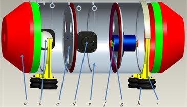
Fig. 15The framework of data acquisition system

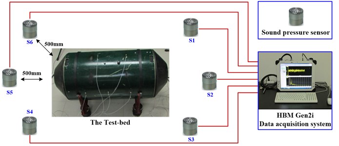
Six sound pressure sensors are used to collect acoustical signals, and they are placed in six different directions of the test bed with a same distance of 500 millimeters. HBM Gen2i data acquisition system is used to collect acoustical data. The framework of the data acquisition system is shown in Fig. 15, and the test parameters are shown in Table 1.

4.2. Acoustical signals of the test bed

As all the sources are working with the given parameters, the mixed acoustical signals are measured by six sound pressure sensors. In the experimental study, the acoustical signals from sensors 2, 3, 4 and 6 are used as mixed signals. Generally, the number of the mixed signals is 1 more than that of sources, which is to guarantee an effective source separation of NLFA and also reduce noise effects of environment, and the directions of these sensors represent a diversified mixing mode of sources.

Fig. 16Waveforms of mixed signals

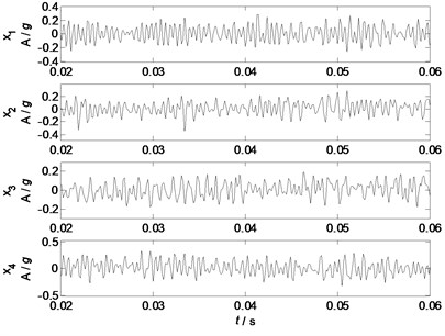
Fig. 17Spectrums of mixed signals

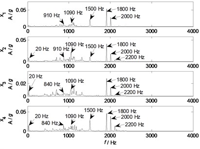
The waveforms and spectrums of mixed signals are shown in Fig. 16 and Fig. 17 respectively. From waveforms in Fig. 16, it is very difficult to identify source features except some periodic waves. While from spectrums in Fig. 17, nearly all the mixed signals contain some major components of 20, 910, 1090, 1500, 1800, 2000, and 2200 Hz, which can be used to identify sources. Generally, independent source information cannot be directly identified from mixed signals as they are coupling together.

4.3. Acoustical source separation

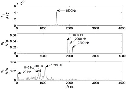
NLFA is applied to separate mixed signals into uncorrelated factors, and 3 factors are extracted from the given mixed signals, whose waveforms and spectrums are shown in Fig. 18 and Fig. 19, respectively. Fig. 18 clearly shows that the waveform of the separated factor ${\mathbf{y}}_1$ has clearly periodic features, and the basic component is a sine wave. The spectrum in Fig. 19 also shows that the separated factor ${\mathbf{y}}_1$ has a major component of 1500 Hz. The waveform of the separated component ${\mathbf{y}}_2$ has a typical feature of a sine wave with amplitude modulation, whose spectrum also clearly shows typical features of 1800, 2000, and 2200 Hz. The waveform of the separated factor ${\mathbf{y}}_3$ has an unclear feature of a sine wave with randomly amplitude modulation, whose spectrum has 4 major components of 20, 870, 910, and 1090 Hz.

Fig. 18Waveforms of separated factors

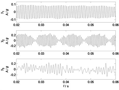
Fig. 19Spectrums of separated factors

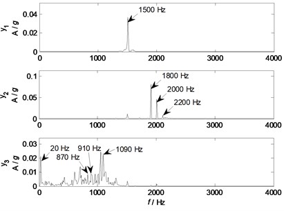
Comparing the spectrums of separated components with parameters of experimental setups, it can be speculated that the separated factor ${\mathbf{y}}_1$ represents a typical feature of source 1 from Loudspeaker I, while the separated factors ${\mathbf{y}}_2$ and ${\mathbf{y}}_3$ represent typical features of source 2 and 3 from loudspeaker II and the motor, respectively. However, this is just based on parameters of experimental setups, and still not a convincing and reliable source identification method.

4.4. Acoustical source identification and validation

To intelligently identify sources from the separated factors, and validate the effectiveness of NLFA for acoustical signals of real mechanical systems, source signals are measured independently by the closest sensors in the condition that only the related source is working with given parameters. The waveforms of independent sources from sensors 1, 4, and 6 for Loudspeaker I, Loudspeaker II, and the motor are shown in Fig. 20, and their corresponding spectrums are shown in Fig. 21.

Comparing waveforms in Fig. 20 and spectrums in Fig. 21 of source signals with that in Fig. 18 and Fig. 19 of separated factors, the waveforms of separated factors are very similar to that of related sources: the separated factor ${\mathbf{y}}_1$ and source ${\mathbf{s}}_1$ have a clear sine wave of 1500 Hz , which well agrees with the experimental setup (1500 Hz) of Loudspeaker I; the separated factor ${\mathbf{y}}_2$ and source ${\mathbf{s}}_2$ have 3 major components of 1800, 2000, and 2200 Hz corresponding to the experimental setup of Loudspeaker II; the separated factor ${\mathbf{y}}_3$ and source ${\mathbf{s}}_3$ have a basic sine wave (20 Hz) with an uncertainty amplitude modulation, which can be interpreted as an eccentric vibration of the motor, and the uncertainty amplitude modulation (840, 910, 1090 Hz) can be caused by rubbing. Therefore, all the major components of source information have been effectively separated from mixed signals by NLFA.

Fig. 20Waveforms of source signals

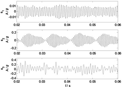
Fig. 21Spectrums of source signals

To quantitatively and intelligently identify sources from separated factors, waveform correlation analysis is used to measure similarity between separated factors and sources. All 3 separated factors are made correlation analysis with all 3 sources, and their correlation coefficients are listed in the correlation matrix ${\mathrm{\Omega }}_W$:

The correlation matrix ${\mathrm{\Omega }}_W$ shows that correlation coefficients between separated factors and related sources are 0.92, 0.92 and 0.72, which indicate high correlation coefficients or high similarity between separated factors and related sources (Liu [32] obtained waveform correlation coefficients of 0.77±0.03 for ECG signals with noises, and Farila [33] obtained waveform correlation coefficients of 0.70±0.09 for non-stationary surface myoelectric signals); while correlation coefficients between separated factors and unrelated sources are all less than 0.13, which indicates that all 3 sources have a good independence property. Therefore, a threshold $\gamma$ can be set as $\gamma \in \text{(0.13,}\text{0.72)}$ (Normally 0.55~0.65) to intelligently identify acoustical sources. Furthermore, high correlation coefficients between separated factors and related sources validate that the effectiveness of NLFA in acoustical source separation and identification.