Electrocardiogram time series forecasting and optimization using ant colony optimization algorithm

Čepulionis, Paulius; Lukoševičiūtė, Kristina

Mathematical Models in Engineering

Browse Journal

Submit article

Published: 30 June 2016

Check for updates

Electrocardiogram time series forecasting and optimization using ant colony optimization algorithm

Paulius Čepulionis¹

Kristina Lukoševičiūtė²

^{1, 2}Kaunas University of Technology, Kaunas, Lithuania

Corresponding Author:

Paulius Čepulionis

Cite the article Download PDF

Downloads 2408

Abstract

The aim of this work is to create the time series dynamic model, which is based on non-uniform embedding in the phase-space. To solve selection of time delays problem efficiently, this paper proposes an ant colony optimization (ACO) way. Firstly, false nearest neighbor method is used for determine the embedding dimension. Secondly, ant colony optimization algorithm is used for non-uniform time delay search. To quicken search speed, roulette wheel selection algorithm distributes ants’ pheromones. Optimization fitness function is the average area of all attractors. Obtained embeddings found by this model are applied in time-series forecasting using radial basis function neural networks. The study is presented in Mackey-Glass and electrocardiogram (ECG) time series forecasting. Prediction results show that the proposed model provides precise prediction accuracy.

1. Introduction

The time series analysis has attracted attention of researchers’ during the last decade [1-3]. It is applied in many fields of science: economic forecasting, stock market analysis, bio-signal analysis, weather forecasting.

In most cases real-world time series are chaotic and nonlinear. These complex chaotic systems exist in many theoretical and practical problems: signal processing, communications, control, social economics and bio-informatics [1, 4, 5]. As the result, chaotic time series prediction is challenge since the structure in their attractors tends to be very intricate and non-uniform [5].

Phase space reconstruction method was introduced by Packard et al. (1980) and mathematically stated as the embedding theorem by Takens (1981). The embedding theorem states that dynamics of a time series can be embedded in the $m$ -dimensional phase space, where $m \geq 2 d + 1$ , and the appropriate choice of a time delay $τ$ and a sufficiently great dimension $d$ can predict the dynamics of chaos. A Number of methods were suggested/used for optimal embedding parameters selection, but none of them is sufficiently effective [1-4].

Non-uniform embedding must be used in order to increase the effectiveness of attractor reconstruction. Non-uniform embedding allows to choose different time-delays for different dimensions and enables a more flexible way to reconstruct the dynamics. However, the investigation becomes more complicated due to the different parameter options [1].

The analysis of the electrocardiogram (ECG) is well-known in the biomedical engineering field. It is important to accurately predict signal since ECG analysis can provide useful information for the detection, diagnosis and treatment of various diseases. For example, ECG monitoring system need to predict future signal and provide disease warning according to diagnosis of the predicted ECG signal [6, 7].

2. Electrocardiogram data

The research data is Electrocardiography (ECG) recordings from Northwestern University (Fig. 1). For investigation, we used a 1-minute length patient’s electrocardiogram, which is diagnosed with Atrial fibrillation (AF), and for prediction the further ECG recording (Fig. 1). AF is the most common type of arrhythmia. An arrhythmia is a problem with the rate or rhythm of the heartbeat and it is one of the most common heart disease among older people. This data has been created for challenge in the “Computers in Cardiology Challenge 2001” with the goal of developing models for forecasting ECG recordings and predicting paroxysmal atrial fibrillation [6].

Fig. 1a) Short electrocardiogram signal, b) full electrocardiogram data

a)

b)

3. Methods

Let $x (t) = \{x (1), x (2), \dots, x (n)\}$ be a time series data were $x$ – scalar at specific time, $t$ – time and $n$ – our time series length. One of study purposes is to find optimal embedding parameters – dimension $d$ and time delays $τ_{i}$ . As mentioned in the introduction, the non-uniform embedding uses different time delays $τ_{i}$ . Vector $υ_{t}$ is reconstructed in the d-dimensional phase space Eq. (1) [1]:

1

υ_{t} = (x (t), x (t - τ_{1}), x (t - τ_{2}), \dots, x (t - τ_{d - 1})) .

In non-uniform embedding there is a combinatorial explosion of the possible settings for $(τ_{1}, τ_{2}, \dots, τ_{d - 1})$ as the dimension $d$ increases. Therefore, the ant colony optimization (ACO) algorithm is used to search for $τ_{i}$ parameters [1-3].

3.1. The false nearest neighbor algorithm

The false nearest neighbor algorithm (FNN) was used to select the optimal dimension. FNN algorithm determines the minimum required dimension for optimal attractor reconstruction. This must be done firstly, because time-delays search is determined by the appropriate dimension [8, 9].

Suppose we have dimension $d$ and distance to the nearest neighbor $y^{r} (n)$ . We calculate the Euclidean distance between $y (n)$ and $y^{r} (n)$ :

2

R_{d}^{2} (n, r) = \sum_{j = 0}^{d - 1} {[x (n + j T) - x^{r} (n + j T)]}^{2} .

Calculate $d + 1$ dimension and distance between $y (n)$ and same nearest neighbor $y^{r} (n)$ using formula:

3

R_{d + 1}^{2} (n, r) = R_{d}^{2} (n, r) + {[x (n + d T) - x^{r} (n + d T)]}^{2} .

Method examines distance difference when moving from the dimensions $d$ to $d + 1$ . Distance difference can be calculated using the Eq. (2) and (3). Wrong neighbor assigned to any neighbor using the formula:

4

\sqrt[2]{\frac{R_{d + 1}^{2} (n, r) - R_{d}^{2} (n, r)}{R_{d}^{2} (n, r)}} = \frac{⌊x (n + d T) - x^{r} (n + d T)⌋}{R_{d}^{2} (n, r)} > R_{t o l},

where $R_{t o l} = 15$ . The second criterion Eq. (5):

5

\frac{R_{d + 1} (n)}{R_{A}} > A_{t o l},

where $A_{t o l} =$ 2 [8, 9].

3.2. Ant colony optimization algorithm

Ant colony optimization (ACO) algorithm is used to efficiently find suitable time-delays. ACO is swarm intelligence method proposed by Dorigo in 1990s and it is widely used to solve NP-hard problems, such as the traveling salesman problem (TSP), the quadratic assignment problem (QAP), the vehicle routing problem (VRP) and the job-shop scheduling problem (JSP) [1, 10]. ACO is inspired by real ant colonies. Ants explore randomly in order to find food. If an ant finds a food, it evaluates and goes back to the nest. During the return travels the ant leaves on the ground pheromone trail. Quantity and quality of the food may determine the quantity of pheromone left on the ground. Other ants can smell the pheromone and follow it with some probability. They tend to choose the paths marked by strong pheromone concentrations. This way, ants can communicate via pheromone and find the optimal path between the food source and their nest. This capability of real ant colony to find optimal paths has led to the definition of artificial ant colonies that can find the optimal solution for hard optimization problems [1, 10, 11]. In this study ants leave their pheromones on chosen time delays if they find a better solution of fitness function, which will be presented in subsequent chapters.

3.3. Roulette wheel selection algorithm

For optimal pheromone distribution the roulette wheel selection (RWS) algorithm, also known as fitness proportionate selection method, was used. RWS is an operator used in genetic algorithms [1, 12]. In this study, roulette wheel selection helps ants to choose time-delays. Firstly, time delays get the same chance of being selected $p = 1 / M a x Τ$ , where $M a x Τ$ is maximum amout of time delay. But when ants find a better solution of fitness function, ants leave their pheromones on the selected time delays ${P (τ}_{j}) = {P (τ}_{j}) + p h$ , where $p h$ is pheromone left by ant.

In the following iterations ${P (τ}_{j})$ is evaluated based on ant pheromones and heuristics values:

6

{P (τ}_{i}) = \{\begin{array}{l} {P (τ}_{i}) = \frac{{P (τ}_{i})}{\sum_{k = 1}^{M a x Τ} {P (τ}_{k})}, & τ \in \{1,2, \dots, M a x Τ\}, \\ 0, & e l s e . \end{array}

3.4. Fitness function

K. Lukoseviciute and M. Ragulskis proposed the hypothesis that “the fitness function is constructed in such a way that it represents the spreading of the attractor in the delay coordinate space” [13]. In this study, we decided to calculate the arithmetic average of the attractors plot as fitness function for each ant. Firstly, fitness function counted each attractor’s surface and then the arithmetic mean of them all. If attractor area is greater than previously known, ants leave their pheromones on the selected time delays and saves best time delays.

3.5. Radial basis function neural network

Eventually, Radial basis function (RBF) neural network was used to forecast data. RBF emerged as a variant of artificial neural network in late 80’s and nowadays it is often used [14, 15]. Basically RBF network is composed of artificial neurons and can be organized into several layers as shown in Fig. 2.

Fig. 2RBF network

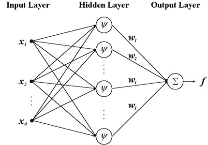
An RBF network is a three-layer feedforward architecture with an input layer, a hidden layer and an output layer. Hidden layer is a single layer of nonlinear processing units. The RBF network input-output relationship:

7

y = \sum_{k = 1}^{N} w_{k} φ (u, t_{k}) + w_{0},

where $N$ is the number of hidden layer nodes (neurons); the term $φ (u, t_{k})$ is the $k$ th Radial basis function that computes the distance between an input vector $u$ and its own center $t_{k}$ . The scaling factor $w_{k}$ in Eq. (8) represents a weight that connects the $k$ th hidden node to the output node of the network. The constant term $w_{0}$ in Eq. (8) represents a bias. The Gaussian form is used in RBF:

8

φ (u, t_{k}) = \exp (- \frac{1}{σ_{k}^{2}} {‖u - t_{k}‖}^{2}), k = 1,2, \dots, N,

where $σ_{k}$ is the width, and $‖u - t_{k}‖$ denotes the Euclidean distance between $u$ and its own center $t_{k}$ .

Thus, substituting Eq. (8) into Eq. (7), we may formulate input-output mapping realized by a Gaussian RBF network as follows:

9

y = \sum_{k = 1}^{N} w_{k} \exp (- \frac{1}{σ_{k}^{2}} {‖u - t_{k}‖}^{2}) + w_{0} .

From a design point of view, the training of RBF networks is to find the number of hidden neurons and output vector with good accuracy. RBF neural network is trained until the training error is improving [14-16].

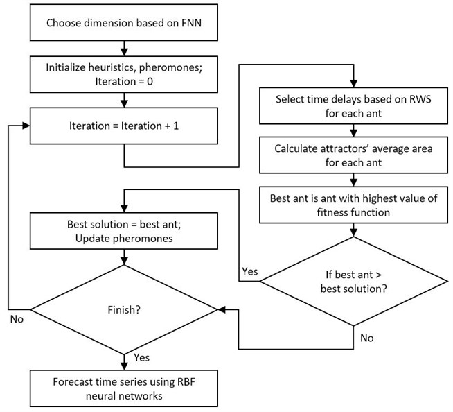
Fig. 3The time series reconstruction to non-uniform time delay space and RBF forecasting algorithm

4. Results

Forecasting was carried out for two-time series. The first one is a classical Mackey-Glass chaotic time series. The second one is ECG time series.

Baseline variables were used same for both time series: number of ants – 30, pheromone size – 0.01, attractors were divided into the 50 pieces to calculate the area, maximum number of iterations for ACO algorithm – 500. The maximum time delay has been selected in view of the time series seasonality or using no more than 20 % of the chaotic time training data.

4.1. Mackey-Glass results

In order to mathematically illustrate the effectiveness of our proposed method, a benchmark chaos time series is used as the first study. The Mackey-Glass time series (Fig. 4) Eq. (10) was chosen because it is the traditional chaotic time series, which is often used by other authors:

10

x (t + 1) = 0.2 \frac{x (t - 17)}{1 + x {(t - 17)}^{10}} + (1 - 0.1) x (t) .

Fig. 4Mackey-Glass time series

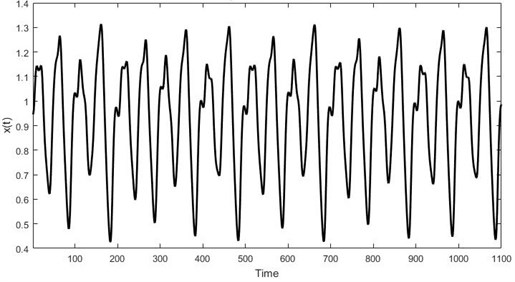
Firstly, false nearest neighbor algorithm determined that a minimum dimension is 4 and ant colony optimization algorithm has found the highest fitness function with value $F (8,91,97) = 3,2008$ and time delays ${τ_{1} = 8; τ_{2} = 91; τ_{3} = 97}$ . Secondly, RBF neural network is trained using 500 Mackey-Glass time series elements and the remaining 500 elements are used to evaluate prediction. Neural network epochs of training – 61, spread – 2.3 and achieved a training error – 3.48×10^-11.

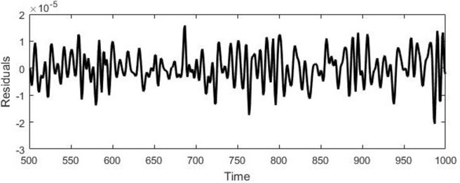
Fig. 5a) Real Mackey-Glass data, b) RBF forecast, c) Residuals

a)

b)

c)

Student’s t-test confirmed that the errors are distributed along the zero $(p =$ 0), Kolmogorov-Smirnov test denied hypothesis that the error is dependent on the data ( $p =$ 1). The forecasting results are shown in Fig. 4. It can be seen from Table 1 that the forecasting output can predict the time series with small residuals.

Table 1Comparison of different methods for the prediction of Mackey-Glass time-series

Model	RMSE
FBBFNT EGP & PSOUM-IHS [17]	4,8876×10^-13
FBBFNT EGP & ABC-OPSOP [18]	1,3534×10^-10
FBBFNT EIP & HBFOA [19]	1,863×10^-9
Our proposed method	5,8821×10^-6
Fuzzy inference system with non-uniform embedding [13]	3,497×10^-4
GADNN [20]	4,7×10^-4
FNT [21]	2,7×10^-3
Neural tree model [22]	2,6×10^-2
HyFIS [23]	4,2×10^-3
Classical RBF [24]	1,14×10^-2
K-nearest neighbor [25]	1,94×10^-2
FuNN [26]	7,1×10^-2
Fuzzy system [27]	8,16×10^-2
Linear model [28]	5,503×10^-1
ARMA [29]	8,43×10^-1

4.2. ECG results

False nearest neighbor algorithm determined that a minimum dimension is 9. Ant colony optimization algorithm has found the highest fitness function with value 9.1365×10⁵ and time delays ${τ_{1} = 1; τ_{2} = 4; τ_{3} = 5; τ_{4} = 309; τ_{5} = 337; τ_{6} = 343; τ_{7} = 344; τ_{8} = 374}$ .

Vector of 8340 points was used in forecast. This vector consists 50 seconds of electrocardiogram. RBF neural network parameters: Spread – 927.5, Neural network epochs of training – 137 and achieved a training error – 5.391×10^-7.

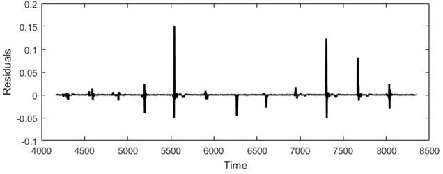
Model prediction is checked according to errors. Student t test confirmed the hypothesis that the errors are distributed along the zero. MAPE of our proposed algorithm – 0,0492 %, RMSE – 6.6×10^-3.

Fig. 6a) Real ECG data, b) RBF forecast, c) Residuals

a)

b)

c)

5. Conclusions

Electrocardiogram forecasting is important to health monitoring system. Due to the stochastic and nonlinear characteristics of ECG system, it is difficult to correctly reconstruct the characteristics of the system. A new training method for RBF neural networks is proposed in this paper and tested with ECG data and Mackey-Glass time series.

The validity of this method is proved by the prediction of Mackey-Glass chaos time series and ECG data. Mackey glass benchmark revealed that method chooses parameters effectively and forecasts time series with small residuals as compared with others methods. The model accurately predicts 25 seconds (4170 elements) ahead of ECG data and is a reliable method for time series forecasting.

References

Shen M., Chen W.-N., Zhang J., Chung H. S.-H., Kaynak O. Optimal selection of parameters for nonuniform embedding of chaotic time series using ant colony optimization. Cybernetics, Vol. 43, Issue 2, 2013, p. 790-802.

Search CrossRef
Zhang J., Chung S.-H., Lo W-L. Chaotic time series prediction using a neuro-fuzzy system with time-delay coordinates. Knowledge and Data Engineering, Vol. 20, Issue 7, 2008, p. 956-964.

Search CrossRef
Brockwell P. J., Davis R. A. Introduction to Time Series and Forecasting. Springer Science and Business Media, 2006.

Search CrossRef
Pecora L. M., Moniz L., Nichols J., Carrol T. L. A unified approach to attractor reconstruction. Chaos: An Interdisciplinary Journal of Nonlinear Science, Vol. 17, Issue 1, 2007, p. 013110.

Search CrossRef
Su L. Y. Prediction of multivariate chaotic time series with local polynomial fitting. Computers and Mathematics with Applications, Vol. 59, Issue 2, 2010, p. 737-744.

Search CrossRef
Moody G., Goldberger A., McClennen S., Swiryn S. Predicting the onset of paroxysmal atrial fibrillation: the computers in cardiology challenge 2001. Computers in Cardiology, Vol. 28, Issue 1, 2001, p. 113-116.

Search CrossRef
Tang X. Novel Remote ECG Real-Time Monitoring System. M.Phil. Thesis, Hong Kong University of Science and Technology, 2009.

Search CrossRef
Rhodes C., Morari M. False-nearest-neighbors algorithm and noise-corrupted time series. Physical Review, Vol. 55, Issue 5, 1997, p. 6162-6170.

Search CrossRef
Mezeiová K., Krakovská A. Choice of measurement for phase-space reconstruction: decision based on false nearest neighbors method. Journal of Complex Systems, 2011, p. 55-58.

Search CrossRef
Zhao F., Dong J., Li S., Sun J. An improved ant colony optimization algorithm with embedded genetic algorithm for the traveling salesman problem. Intelligent Control and Automation, 2008, p. 7902-7906.

Search CrossRef
Al-Qaheri H. Digital watermarking using ant colony optimization in fractional Fourier domain. Journal of Information Hiding and Multimedia Signal Processing, Vol. 1, Issue 3, 2010, p. 179-189.

Search CrossRef
Arabas J., Bartnik L., Opara K. DMEA – an algorithm that combines differential mutation with the fitness proportionate selection. Differential Evolution (SDE), 2011, p. 1-8.

Search CrossRef
Lukoseviciute K., Ragulskis M. Evolutionary algorithms for the selection of time lags for time series forecasting by fuzzy inference systems. Neurocomputing, Vol. 73, Issue 10, 2010, p. 2077-2088.

Search CrossRef
Packard N. H., Crutch J. P., Farmer J., Shaw R. Geometry from a time series. Physical Review Letters, Vol. 45, 1980, p. 712-716.

Search CrossRef
Ma N., Lu C., Zhang W. J., Wu X. H. Application of parallel RBF network on iterative prediction of chaotic time series. Chaos-Fractals Theories and Applications (IWCFTA), 2010, p. 341-345.

Search CrossRef
Haiping D., Nong Z. Time series prediction using evolving radial basis function networks with new encoding scheme. Neurocomputing, Vol. 71, Issues 7-9, 2008, p. 1388-1400.

Search CrossRef
Bouaziz S., Alimi A. M., Abraham A. PSO-based update memory for improved harmony search algorithm to the evolution of FBBFNT’ parameters. Evolutionary Computation (CEC), 2014, p. 1951-1958.

Search CrossRef
Bouaziz S., Dhahri H., Alimi A. M., Abraham A. Evolving flexible beta basis function neural tree using extended genetic programming and hybrid artificial bee colony. Applied Soft Computing, 2016, p. 1-16.

Search CrossRef
Bouaziz S., Alimi A. M., Abraham A. Evolving flexible beta basis function neural tree for nonlinear systems. Neural Networks (IJCNN), 2013, p. 1-8.

Search CrossRef
Jaddi N. S., Abdullah S., Hamdan A. R. A solution representation of genetic algorithm for neural network weights and structure. Information Processing Letters, Vol. 116, Issue 1, 2016, p. 22-25.

Search CrossRef
Chen Y., Yang B., Dong J., Abraham A. Time-series forecasting using flexible neural tree model. Information Sciences, Vol. 174, Issue 3, 2005, p. 219-235.

Search CrossRef
Chen Y., Yang B., Dong J. Nonlinear system modelling via optimal design of neural trees. International Journal of Neural Systems, Vol. 14, Issue 2, 2004, p. 125-137.

Search CrossRef
Kim J., Kasabov N. HyFIS: adaptive neuro-fuzzy inference systems and their application to nonlinear dynamical systems. Neural Networks, Vol. 12, Issue 9, 1999, p. 1301-1319.

Search CrossRef
Cho K. B., Wang B. H. Radial basis function based adaptive fuzzy systems their application to system identification and prediction. Fuzzy Sets and Systems, Vol. 83, 1995, p. 325-339.

Search CrossRef
Qin Z., Tang Y. Uncertainty Modeling for Data Mining: A Label Semantics Approach. Springer, 2014.

Search CrossRef
Kasabov N. K., Kim J., Watts M. J., Gray A. R. FuNN/2 – a fuzzy neural network architecture for adaptive learning and knowledge acquisition. Information Sciences, Vol. 101, Issue 3, 1997, p. 155-175.

Search CrossRef
Lee S. H., Kim I. T. Time series analysis using fuzzy learning. ICONIP: International Conference on Neural Information Processing, Vol. 3, Issue 3, 1994, p. 1577-1582.

Search CrossRef
Lazzús J. A., Salfate I., Montecinos S. Hybrid neural network-particle swarm algorithm to describe chaotic time series. Neural Network World, Vol. 24, Issue 6, 2014, p. 601-617.

Search CrossRef
Box G. E. P., Jenkins G. M. Time Series Analysis: Forecasting and Control. Holdenday, San Francisco, Vol. 22, Issue 2, 1976, p. 199-201.

Search CrossRef

About this article

Received

30 April 2016

Accepted

02 June 2016

Published

30 June 2016

Keywords

non-uniform embedding

ant colony optimization

electrocardiogram

time series forecasting

This is an open access article distributed under the Creative Commons Attribution License, which permits unrestricted use, distribution, and reproduction in any medium, provided the original work is properly cited.