Abstract
Faults in rolling element bearings often cause the breakdown of rotating machinery. Not only the fault type identification but also the fault severity assessment is important. So this paper emphasizes the fault severity assessment. The method proposed in this paper contains two steps: first, identify the fault type based on the combination of empirical mode decomposition (EMD) and fast kurtogram; Second, assess the fault severity. In the first step, the original signal is firstly decomposed into some intrinsic mode functions (IMFs) and the representative IMFs are selected based on correlation analysis, and then the reconstruction signal (RS) is generated; Secondly, the fast kurtogram method is applied to the RS, and the optimum band width and center frequency is obtained. The fault type can be identified based on the fault characteristic frequency marked in the envelope demodulation spectrum. In the second step, the energy percentage of the most fault-related IMF is chosen as an indicator of the fault severity assessment. Experimental data of rolling element bearings inner raceway fault (IRF) with three severities at four running speeds were analyzed. The results show that the IRF identification and fault severity assessment is realized. The breakthrough attempt provides the great potential in the application of condition monitoring of bearings.
1. Introduction
As an important part of rotating machinery, rolling element bearing is also one of the most common fault sources of equipment. In the past decades, some faults associated with rolling element bearings had led to severe damage and great economic loss [1, 2]. Hence, it is very necessary to detect and diagnose these faults at an early stage.
As is known to many, the local defect on the surface of rolling element bearings will produce a series of periodic impacts when every rolling element passes through the damage position. This may excite resonances in the bearings and machine. Meantime, modulation signals, e.g., amplitude modulation caused by inner raceway or outer raceway faults, and pulse modulation caused by rolling element fault, will appear [3]. Generally, these faults can be identified through characteristic frequency, namely modulation frequency [4, 5]. However, the low frequency modulation signals are usually carried by high frequency resonance signals, and can be contaminated easily by background noise. Therefore, the key of signal processing is to enhance the impulsiveness of the signal, thus improving the signal-to-noise ratio (SNR) [6]. The characteristic frequency can be extracted and adopted as key indicators in identifying the bearings faults when signals are enhanced and separated from other mechanical components and background noise.
Vibration signals collected from bearings carry a wealth of useful information on machine conditions. Vibration measurement and analysis have been widely used in bearings diagnostics. Over the past decades, various signal analysis methods based on vibration signals for faults diagnosis of rotating machinery have been proposed. Burchill [7] presented the method of resonance demodulation to diagnose the fault of rolling element bearings in the 1970s. The SPM Company later developed an instrument to detect rolling element bearings faults based on the measurement of resonant responses of an accelerometer excited by the faults [8]. However, the effectiveness of this method depends on how well the vibration signal is pre-processed, and what de-noising method is adopted. On the one hand, it is usually difficult to gain a clear envelope spectrum when the background noise can’t be properly separated from the original signal. On the other hand, the resonance frequency, chosen as center frequency, is not always optimal [9]. With the tireless efforts of many researchers, many advanced signal processing techniques were introduced to deal with such impacting signals in the past few decades. These include, wavelet transform [10, 11], multiwavelet [12], empirical mode decomposition (EMD) [13-16], Hilbert-Huang transform (HHT) [17], and Local mean decomposition [18, 19]. Thanks to the advantages of these, such as high capability of nonlinearity identifications, high immunity to additive Gaussian noise, spectral kurtosis (SK) was developed. Antoni and Randall made a significant promotion to SK technique [20-22]. In particular, Antoni [23] proposed a fast algorithm for computing the kurtogram and provided a good application in rolling element bearings faults diagnosis. This was achieved by providing the optimal center frequency and band width. However, high frequency noises may not be separated correctly or some important information may be left out [24], especially when the fault is relatively serious. Therefore, it is necessary to adopt effective methods to improve the signal-to-noise ratio (SNR) before using SK. EMD proposed by Huang et al [25] can decompose a signal into a sum of intrinsic mode functions (IMFs) which reflect the local characteristic of the signal. The frequency band for each IMF ranges from high to low and changes with the original signal itself. The characteristic information of the original signal can be extracted more accurately and effectively based on each IMF, which will contribute to a high SNR. However, many researchers focus on fault type instead of fault severity when using EMD method. So this paper attempts to assess the fault severity by EMD after identifying the fault type.
According to the discussions above, in this paper, a new method combining EMD and Fast Kurtogram is applied to rolling element bearings inner raceway fault diagnosis. Firstly, the raw acceleration vibration signal measured from detective bearings is decomposed by EMD and some IMF components are obtained. Secondly, the representative IMFs containing fault information are selected based on the correlation analysis, and the reconstruction signal (RS) is generated by the addition of the representative IMFs. Thirdly, the optimum bandwidth and center frequency of the RS is provided by Fast Kurtogram. The fault characteristic frequency is then marked in the envelope spectrum and the fault type is identified. Finally, the energy percentage of the most fault-related IMF from the representative IMFs is chosen as the indicator for fault severity assessment. Experimental data of rolling element bearings inner raceway fault (IRF) with three severities at four running speeds were analyzed. The results showed that the diagnosis approach combining EMD and Fast Kurtogram had good effectiveness in IRF identification and severity assessment.
The paper is organized as follows. Section 2 is dedicated to the related work, including the brief introduction of EMD and its numerical simulation; the correlation analysis; the IMF energy percentage; and the definition and algorithm of Fast Kurtogram method. In Section 3, the fault signatures of rolling element bearings are introduced. In Section 4, the experimental rigs and data records are described. In Section 5, the fault diagnosis method for rolling element bearings based on EMD and Fast Kurtogram is proposed. Section 6 gives the application of the proposed method. Finally, the conclusions of this paper are given in Section 7.
2. Related work
EMD is a self-adaptive signal processing method and has a high robustness nature, which makes it especially suitable for the non-stationary and non-linear signals analysis [25], and has been widely used in bearings fault diagnosis [26, 27]. Spectral Kurtosis (SK) is a powerful tool for detecting the presence of transients in a signal, even when they are buried in strong additive noise, by indicating in which frequency bands they are taken place. Kurtogram considers a variety of bandwidths and central frequencies. Fast Kurtogram, a visualized kurtosis fast algorithm, makes spectral kurtosis a powerful analysis tool for non-stationary signals.
2.1. EMD method
The EMD method is based on such a simple assumption that any signal consists of different simple oscillatory modes. The definition and algorithm of EMD has been described in detail by Huang et al. [25]. According, to the EMD algorithm, any original signal x(t) can be represented by a sum of IMFs:
where ci(t) denotes ith IMF and rn(t) is the final residue after allIMFs are extracted. Each IMF should satisfy the following two conditions [27]:
a) In the whole data set, the number of extrema and the number of zero-crossings must either be equal or differ at most by one.
b) At any point, the mean value of the envelope defined by local maxima and the envelope defined by the local minima is zero.
The IMFs can be achieved by the following steps [25]:
(1) Find out all the local extreme values of the original signal and connect the local maxima and minima respectively to construct the upper and lower envelopes by a cubic spline interpolation.
(2) Specify the mean of the two envelopes as m1(t), and the difference between x(t) and m1(t) is designated as h1(t), i.e.:
Ideally, h1(t) will be the first component of x(t) if it is an IMF.
(3) If h1(t) is not an IMF, take it as the new original signal and repeat the steps (1)-(2); then a new mean m11(t) is calculated, so does the h11(t), i.e.:
Judge whether h11(t) is an IMF, if not, repeat sifting, i.e. up to k times, until h1k(t) becomes an IMF, i.e.:
Set h1k(t) as c1(t) (the first IMF), i.e.:
(4) Subtract c1(t) fromx(t), the first residual r1(t) is got:
(5) Treat the residual r1(t) as the original signal, and repeat the steps (1)-(4) ntimes and the other IMFs (ci, i=2,…,n.) will be obtained .The EMD decomposition will be stopped until the residual rn(t) becomes a monotonic function:
Finally, the original signal x(t) is decomposed into n-emprical modes c1,…, cn including different frequency bands ranging from high to low and a residual rn(t) which is the mean trend of x(t).
2.2. Numerical simulation
To certify the ability of EMD to decompose the original signal into a sum of IMFs which can reveal the internal structure of the signal, a simulated signal containing multiple frequency components and some normal distributed random noise is constructed as Eq. (8):
where f1=100 Hz, f2=200 Hz, f1=300 Hz, and φ(t) is the Gaussian white noise.
The IMFs gained by EMD and the corresponding frequency spectrum are illustrated in Fig. 1. According to Fig. 1, it is obvious that the three frequency components belonging to the signal have been extracted successfully by EMD and are clearly shown in the first two IMFs. However, the last six IMFs are irrelevant with the original signal. These pseudo components are generated by over decomposition of EMD and may interfere with further signal processing such as feature extraction and fault diagnosis. Therefore, the IMF selection method is necessary to remove the pseudo components [28].
Fig. 1Demonstration of the IMFs
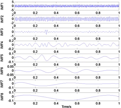
a) Waveforms in time domain
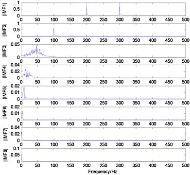
b) The corresponding frequency spectrums
2.3. IMF selection based on correlation analysis
EMD is based on the local characteristic timescales of a signal and can self-adaptively decompose the complicated signal into some IMFs reflecting the oscillatory mode embedded in the signal. However, in many cases, the high frequency components obtained from EMD are removed directly as noise, which may leave out some important information. In particular, for rolling element bearings, the impulsive signals related to the faults usually lie in the high frequency band. Therefore, selecting appropriate IMFs from EMD results is very necessary for faults diagnosis in different conditions.
Because of interpolation error, boundary effects and over decomposition of EMD, the pseudo components, which have nothing to do with the original signal, may appear in EMD. This may interfere the diagnosis results. So a method should be taken to find out these pseudo components and remove them. Wang et al. [28] introduced the correlation-based method which will be used in this paper.
Ideally, a signal s(t) consists of a series of IMFs ci(t), which are all embedded in the original signal in theory, i.e.:
In practice, considering the fact that the pseudo components may be produced by EMD, the form of Eq. (9) will be changed as follows:
where ¯ci(t) and xj(t) denotes the true and pseudo IMF respectively.
The cross-correlation coefficient between s(t) and ci(t) can be calculated by Eq. (11):
=Rci,¯ci(τ)+∑nj=1,j≠iRcj,¯ci(τ)≈Rci,¯ci(τ)≈Rci(τ).
Because of the orthogonality of IMFs, Eq. (12) can be established:
Obviously, the pseudo components have little correlation with the original signal, that is, the correlation coefficient between s(t) and xk(t) should be close to zero as Eq. (13) shows:
In conclusion, the correlation coefficient between the original signal and the true IMFs is approximate to the auto-correlation coefficient of the true IMFs themselves, while the correlation coefficient between the original signal and the pseudo IMFs is very small, close to zero. Therefore, it is very easy to distinguish the true IMFs and pseudo components.
2.4. IMF Energy percentage
The energy of the vibration signal will change with the conditions in which the bearings is operating. From Section 2.1, it can be seen that EMD can decompose the vibration signal into a series of IMFs which has the frequency band from high to low. So each IMFi (i=1,…, n) component corresponds to an energy Ei (i=1,…, n) which forms an energy distribution in the frequency domain, and then the corresponding IMF energy percentage is designated as:
To demonstrate that energy distribution of IMF components will vary from the conditions in which the bearings is operating, four cases including normal, inner raceway fault (IRF), outer raceway fault (ORF), ball fault (BF) are considered. The vibration acceleration signals corresponding to each case is decomposed firstly by EMD. Next, the IMF energy percentages are calculated. Fig. 2 shows the original vibration signals and its first two IMFs of four cases respectively. The corresponding energy percentage is shown in Table 1.
Table 1The energy percentage of the first two IMFs of four cases
Cases | Normal | IRF | BF | ORF |
IMF1 | 0.2304 | 0.7665 | 0.8432 | 0.9574 |
IMF2 | 0.2627 | 0.1495 | 0.0759 | 0.0237 |
From Table 1, it is seen that the IMFs energy distribution of four cases is different distinctly. For IMF1, the energy percentage increases from Normal to ORF, while, for IMF2, it is just the reverse. In particular, the energy percentage will change suddenly from the normal to the fault, such as the energy percentage of IMF1 being just 0.2304 in the normal, while it becomes 0.9574 when the bearings has ORF. So it can be concluded that energy percentages of IMFs based on EMD can basically reflect the work condition of the bearings.
Fig. 2The original vibration signal and its first two IMFs
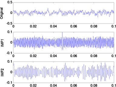
a) Normal
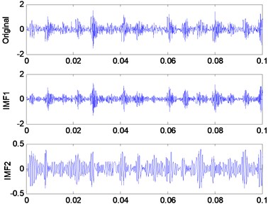
b) IRF
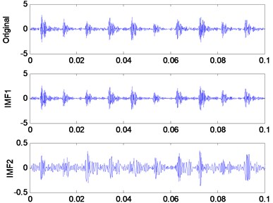
c) ORF
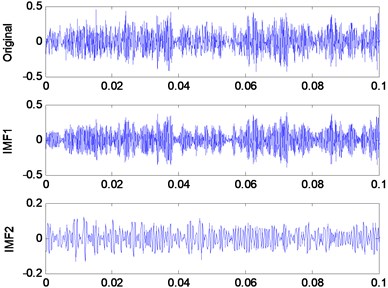
d) BF
2.5. Fast Kurtogram
Kurtogram appeared firstly in [20], which derived from the so called SK. SK is very sensitive to the transient components in signal, and can also indicate accurately their types. According to Antoni [21], considering any stationary random process Y(t), its Wold-Cramer representation can be defined as follows:
where H(t,f) stands for the complex envelope of Y(t) at time t and frequency f, and dX(f) refers to the spectral increment associated with X(t).(X(t), it is a process which has a flat spectrum everywhere).
The fourth-order spectrum cumulant of Y(t) is expressed as follows:
where S(f) denotes the instantaneous spectrum moment, i.e.:
Thus, the SK can then be obtained by the normalized fourth-order cumulant:
In practical applications, the vibration signalsx(t) measured from rotating machinery usually contain two parts: the fault-related signal f(t) and the additive noise n(t), i.e.:
Therefore, the SK of x(t) can be given as follows:
where ρ(f)=Sn(f)/Sf(f) is the noise-to-signal ratio, Sn(f) and Sf(f) is the power spectral density of n(t) and f(t) respectively.
According to Eq. (20), it can be concluded that when the noise is very weak, i.e. ρ(f) is quite small, Kx(f)≈Kf(f); whilst the noise is very strong, i.e. ρ(f) is very large, and Kx(f) is close to zero. Therefore, the whole frequency domain can be detected when the SK is applied locally to different frequency bands, which indicates that the SK can not only detect effectively fault-related signals, but also locate their types in the frequency domain.
Fast Kurtogram, as the name suggests, represents a kurtosis vs frequency diagram produced by a fast algorithm. This fast algorithm [23] bases on the assertion that “each type of transient is associated with an optimal dyad (frequency/frequency resolution), which maximizes its kurtosis, and hence its detection”. To learn about dyadic wavelet decomposition algorithm, firstly, the original signal is decomposed into a series of frequency-band signals, the kurtosis value on each frequency band is calculated in the following; Secondly, a kurtosis vs frequency diagram is generated, from which where there is the biggest kurtosis value , and there is the optimal center frequency and bandwidth ;Thirdly, the signal is filtered based on the optimal center frequency and bandwidth ,and demodulated by square enveloping; Finally the characteristic frequency is gained by spectrum analysis and the faults can be diagnosed.
3. Rolling element bearings faults signatures
On the basis of the different vibration characteristics, the faults, emerging in the operation of rolling element bearings, can be classified into two classes: single-point faults and generalized roughness. Single-point faults are surface damage faults and classified into three types: outer raceway fault, inner raceway fault and ball fault. In this paper, single-point faults are what we are interested in. For single-point faults, a series of abrupt impulsive force will be produced when the balls pass over the local damage point. The repetition rate of the impulsive force is solely determined by the rotational speed (when it is constant) as well as the geometry of the bearings. The repetition rate is usually called the fault characteristic frequency, and varies from the type where the fault emerges. There are different fault characteristic frequencies associated with different parts of the bearings, for example, Ball Passing Frequency Outer Race (BPFO), Ball Passing Frequency Inner Race (BPFI), and Ball Fault Frequency (BFF), which are associated with the outer race, the inner race and the ball respectively. These frequencies can be calculated by the following equations:
where d and D denotes the ball diameter and pitch diameter of bearings respectively, fn is the rotor shaft frequency, Z is the number of balls, and θ is the angle of the load from the radial plane. The geometry of the rolling element bearings is shown in Fig. 3. In Fig. 3(b), besides the three parameters d, D, θ, the De, Di is the external diameter and inner diameter respectively.
Fig. 3The geometry of the rolling element bearings
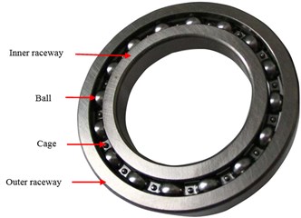
a) The picture
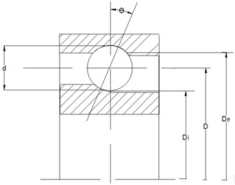
b) The model
4. Experimental rigs and data records
The vibration datasets used in this paper were downloaded from the Case Western Reserve University Bearings Data Center [29]. The basic layout of the test rig is shown in Fig. 4. It consists of a 2 hp, a three-phase induction motor driving a shaft on which a torque transducer and encoder are mounted. Torque is applied to the shaft via a dynamometer and electronic control system. The bearings used in this experiment were 6205-2RS JEM SKF deep groove ball bearings. The specifications are shown in Table 2. Single point faults ranging in diameter from 0.007 to 0.021 inches (0.1778 mm, 0.3556 mm, 0.5332 mm) were introduced to the drive-end bearings of the motor using electro- discharge machining (EDM). The faults were set separately on the rolling elements, inner raceway and outer raceway, and each faulty bearings was reinstalled on the test rig. Tests were carried out under different loads ranging from 0 hp to 3 hp with an 1hp increment which corresponds to 1797, 1772, 1750, and 1730 rpm respectively. Table 3 shows the corresponding fault characteristic frequencies at different running speeds. Vibration data measured in the vertical direction on the housing of the drive-end bearings (DE) were collected using an acquisition system at a sampling frequency of 12 kHz for different bearings conditions.
Fig. 4The bearings test rigs
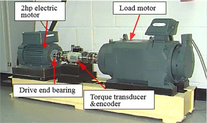
Table 2The specification of test bearings
Parameters | De (mm) | Di (mm) | d (mm) | D (mm) | Z | cosθ |
Size | 51.98 | 24.99 | 7.94 | 39.02 | 9 | 0.9 |
Table 3The BPFI at different running speeds
Running speeds (rpm) | 1730 | 1750 | 1772 | 1797 |
BPFI (Hz) | 156.1 | 157.9 | 159.8 | 162.1 |
5. Faults diagnosis of rolling element bearings based on EMD and Fast Kurtogram
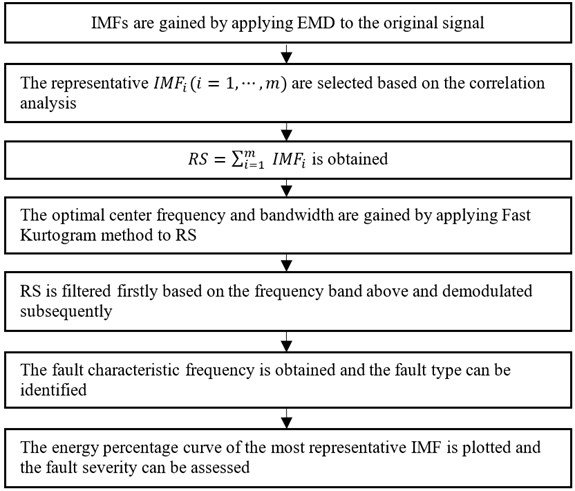
According to the above analysis in Section 2, the true and fault-related IMFs can be reserved, whilst the pseudo components can be removed based on correlation analysis. The work conditions of the bearings can be basically reflected by the energy distribution of IMFs. In this paper, the reconstruction signal (RS), based on the addition of the reserved IMFs, will be as the original signal of the Fast Kurtogram method, which will be used to identify the fault type. The energy percentage of the most fault-related IMF, selected from the reserved IMFs, will be used to assess the fault severity. The flow chart of rolling element bearings faults diagnosis method based on the combination of EMD and Fast Kurtogram is shown in Fig. 5.
The fault diagnosis method is given as the following:
(1) The original vibration signal is decomposed into a series of IMFs and the representativeIMFi (i=1,…, m), which include the most dominant fault information, are selected based on the correlation analysis.
(2) Reconstruction of the selected IMFs, namely RS=∑mi=1IMFi which will be as the original signal of the Fast Kurtogram method.
(3) RS is decomposed into a series of frequency-band signals and the kurtosis values on each frequency band are calculated.
(4) A kurtosis vs frequency diagram is generated, from which the optimal center frequency and bandwidth is gained.
(5) RS is filtered based on the optimal center frequency and bandwidth and demodulated by square enveloping.
(6) The fault characteristic frequency is obtained by spectrum analysis and the fault type can be identified.
(7) The energy percentage curves of the most representative IMF are plotted in different work conditions and the fault severity can be assessed.
Fig. 5The flow chart of the rolling element bearings fault diagnosis method based on the combination of EMD and Fast Kurtogram
6. Application
6.1. Bearings fault diagnosis
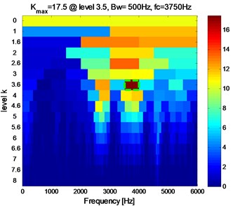
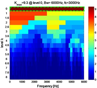
The experimental rigs and data records are described in detail in Section 4. In this paper, the inner raceway fault with three severities (0.1778 mm, 0.3556 mm, 0.5332 mm) at four running speeds (1797, 1772, 1750, 1730 rpm) are considered. The sampling frequency is 12 kHz and the data length is 65536.The vibration signals with four cases (case_0: Normal, case_1: 0.1778 mm, case_2: 0.3556 mm, case_3: 0.5332 mm) for IRF at 1730 rpm are decomposed into 16 IMFs by EMD firstly, and the cross-correlation coefficient (R) between IMFi, i=1,…, 16 and the original signal are calculated subsequently. Table 4 shows the result of the first 8 IMFs. It is known that, the correlation degree is low at |R|<0.3 [30], which can be neglected. It can be seen from Table 4 that the first three IMFs for case_1 (0.2703 ≈ 0.3), the first two IMFs for case_2, and the first IMF for case_3, satisfy the condition of |R|≥0.3. So the representative IMFs for the three cases are the first three, the first two, and the first component(s) respectively. The reconstruction signals (RS) are generated by the addition of the representative IMFs for each case. The results applying Fast Kurtogram method to RS for each case are shown as Fig. 6, and the corresponding envelope analysis are shown in Fig. 7, Fig. 8, and Fig. 9 respectively. The maximum kurtosis value Kmax, the optimum bandwidth Bw and the optimum center frequency fc of the four cases are shown in Table 5. In Fig. 7(c), Fig. 8(c), Fig. 9(c), the characteristic frequencies (154.9 Hz, 155.9 Hz, 155.6 Hz) and their multiplications are marked, and this indicates clearly the inner raceway fault (BPFI=156.1 Hz at 1730 rpm in Table 3).
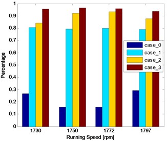
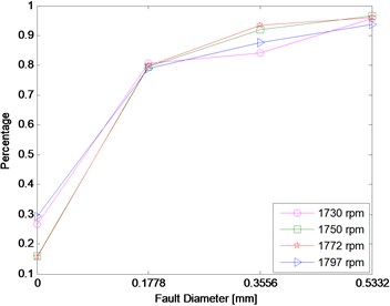
It is can be seen from Table 4 that the cross-correlation coefficient between the first IMF (IMF1), and the original signal, for all the three cases, is the highest in the representative IMFs selected above. This indicates that the IMF1 is the most fault-related component in all IMFs decomposed by EMD. So the energy percentage of IMF1 is selected as the indicator of the fault severity assessment. To make the results convincing, in this experiment, three cases (case_1: 0.1778 mm, case_2: 0.3556 mm, case_3: 0.5332 mm) for IRF, and case_0 for the normal at four running speeds (1797, 1772, 1750, 1730 rpm), 16 cases in total (as Table 6), are considered. The length of data for each case is 10240 which is divided into 10 groups with the length of 1024. For each group of data, it is decomposed into 10 IMFs by EMD, and the energy percentage of each IMF is also calculated. Similarly, the energy percentages of each IMF for the other 9 groups can be gained as well. The final result is the average of that of 10 groups of data for each case. Table 6 shows the energy percentage of IMF1 for all the cases. The corresponding bar chart and the trend curve are shown in Fig. 10. As is shown in Fig. 10, it is obvious that the energy percentage of IMF1 increases with the fault severity, meaning the fault severity becoming more serious when the energy percentage of IMF1 increases. The change is relatively smooth from a light fault to a heavy fault, but it changes sharply from normal to the fault, such as, at 1750 rpm, the percentage is just 0.1585 in case_0, while it becomes 0.7949 which is more than five times of the former in case_1. Furthermore, the results are similar for all four running speeds, which may indicate to a certain extent that the result is not affected by the running speed of the bearings.
Fig. 6The Kutogram of RS at 1730 rpm
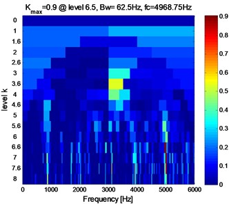
a) Case_0
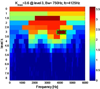
b) Case_1
c) Case_2
d) Case_3
According to the application to the inner raceway fault, it demonstrates the effectiveness of the proposed method in the rolling element bearings inner raceway fault type identification and severity assessment. This method shows the great potential in the application of condition monitoring of bearings. It provides us a possibility to judge whether there is a defect on bearing or not and predict the trend of the faults by monitoring the energy percentage of IMF1. For instance, we can try to calculate the threshold of the energy percentage of IMF1 by a certain amount of experimental data of the normal bearings at a certain condition. If the monitoring result exceeds the threshold, the monitored bearing may have a fault. Further, if the monitoring result becomes more and more big, it indicates that the bearing gets worse and we need to replace it.
Table 4The cross-correlation coefficient between the original signal and IMFi
cases | IMF1 | IMF2 | IMF3 | IMF4 | IMF5 | IMF6 | IMF7 | IMF8 |
case_1 | 0.8552 | 0.3750 | 0.2703 | 0.1794 | 0.0366 | 0.0173 | 0.0035 | 0.0000 |
case_2 | 0.8384 | 0.4777 | 0.2291 | 0.1202 | 0.0720 | 0.0398 | 0.0143 | 0.0000 |
case_3 | 0.9681 | 0.1536 | 0.1062 | 0.1436 | 0.0591 | 0.0182 | 0.0032 | 0.0000 |
Table 5The maximum kurtosis, the optimum bandwidth and center frequency of four cases
cases | case_0 | case_1 | case_2 | case_3 |
Kmax | 0.9 | 3.6 | 17.5 | 9.3 |
Bw (Hz) | 62.5 | 750 | 500 | 6000 |
fc (Hz) | 4968.75 | 4125 | 3750 | 3000 |
Table 6The energy percentage of IMF1 in different conditions
cases | 1730 (rpm) | 1750 (rpm) | 1772 (rpm) | 1797 (rpm) |
case_0 | 0.2675 | 0.1585 | 0.1580 | 0.2938 |
case_1 | 0.8071 | 0.7949 | 0.7993 | 0.7907 |
case_2 | 0.8431 | 0.9210 | 0.9348 | 0.8763 |
case_3 | 0.9570 | 0.9656 | 0.9602 | 0.9380 |
Fig. 7IRF in case_1 at 1730 rpm

a) RS

b) The envelope

c) The envelope spectrum
6.2. Comparison with Hilbert envelope demodulation
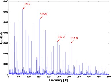
In order to verify the superiority of the proposed method in fault identification, when analyzing the vibration signal shown above, another signal processing technique, envelope demodulation based on Hilbert transform has been applied too, but it did not extract the fault characteristics effectively. For instance, after applying Hilbert envelope demodulation method to the vibration signal at case_1 (0.3556 mm) for IRF at 1730 rpm, the result is shown in Fig. 11. As shown in Fig. 11, although the IRF characteristic frequency (155.9 Hz) and its multiplication (311.8 Hz) can be extracted, there exists some conspicuous and unfathomed frequency components, such as 69.5 Hz and 242.2 Hz marked in Fig. 11, which may easily interfere with diagnostic results and even possibly lead to the wrong ones. By contrast, the characteristic frequencies shown in Fig. 7(c), Fig. 8(c), Fig. 9(c), are very prominent, and the other frequency components are relatively weak which will not affect the diagnostic results.
Fig. 8IRF in case_2 at 1730 rpm

a) RS

b) The envelope

c) The envelope spectrum
Fig. 9IRF in case_3 at 1730 rpm

a) RS

b) The envelope

c) The envelope spectrum
Fig. 10The percentage of IMF1 in different conditions
a) The bar char
b) The trend curve
Besides, another superiority of the proposed method is that it can be not only used to identify the fault patterns but also to assess the fault severities which is also essential for condition monitoring of bearings. To indicate the different severities of fault, a representative indicator is needed to show the variation tendency. However, the envelope demodulation based on Hilbert transform just gives the characteristic frequency which is constant for the same fault with different severities. So Hilbert envelope demodulation fails to assess the fault severities. In contrast, the energy percentage of IMF1 is a good indicator for fault severity assessment.
Fig. 11The Hilbert envelope demodulation spectrum
7. Conclusions
This paper proposes a new diagnosis method for inner raceway fault of rolling element bearings based on the combination of EMD and Fast Kurtogram. The main purpose of this method has two: identifying the fault type and assessing the fault severity. By EMD, the vibration signal can be decomposed into a series of IMFs that reflects the local characteristic of the original signal. The pseudo and little fault-related IMFs can be removed based on the correlation analysis. The characteristic information of the original signal can be extracted more accurately and effectively based on the remaining IMFs which are used to generate the RS. The optimal center frequency and band width of the RS can be provided by Fast Kurtogram. The energy percentages of IMFs can basically reflect the work condition of the bearings and can be chosen as an indicator for fault severity assessment. Experimental data about the inner raceway fault of rolling element bearings was analyzed. From the theory analysis and experiment results, it can be concluded that:
1) EMD is a self-adaptive signal processing method that can be applied to nonlinear and non-stationary processes perfectly.
2) The IMF selection based on the correlation analysis contributes to a high SNR.
3) The Fast Kurtogram is a powerful analysis tool of non-stationary signals, which has the ability to detect transients buried in strong background noise.
4) The combination of EMD and Fast Kurtogram successfully identified the fault type and the energy percentage of IMF1 is a good indicator for fault severity assessment.
5) This method shows the great potential in the application of condition monitoring of bearings. It provides us a possibility to judge whether there is a defect on bearing or not and predict the trend of the faults.
References
-
Liu X. F., Bo L., He X. X., Veidt M. Application of correlation matching for automatic bearings fault diagnosis. Journal of Sound and Vibration, Vol. 331, Issue 26, 2012, p. 5838-5852.
-
Jiang F., Zhu Z., Li W., Chen G., Zhou G. Identification and diagnosis of concurrent faults in rotor-bearing system with WPT and zero space classifiers. Journal of Vibroengineering, Vol. 16, Issue 2, 2014, p. 901-912.
-
Xiang J. W., Zhong Y. T., Gao H. F. Rolling element bearings fault detection using PPCA and spectral kurtosis. Measurement, Vol. 75, Issue 11, 2015, p. 180-191.
-
Patel V. N., Pandey R. K. Defect detection in deep groove ball bearings in presence of external vibration using envelope analysis and Duffing oscillator. Measurement, Vol. 45, Issue 5, 2012, p. 960-970.
-
Tsao W. C., Li Y. F., Duc D. L. An insight concept to select appropriate IMFs for envelope analysis of bearings fault diagnosis. Measurement, Vol. 45, Issue 5, 2012, p. 1489-1498.
-
Randall R. B., Antoni J. Rolling element bearings diagnostics – a tutorial. Mechanical Systems and Signal Processing, Vol. 25, Issue 2, 2011, p. 485-520.
-
Burchill R. F. Resonant structure techniques for bearings fault. Proceedings of Mechanical Failure Prevention Group, Gaithersburg, MD, USA, 1972.
-
Zhang Y. X., Randall R. B. Rolling element bearings fault diagnosis based on the combination of genetic algorithms and fast kurtogram. Mechanical Systems and Signal Processing, Vol. 23, Issue 5, 2009, p. 1509-1517.
-
Engja H., Lippe J. Vibration analysis used for detection of roller bearings failure. Norwegian Maritime Research, Vol. 3, 1977, p. 23-33.
-
Shen C. Q., Liu F., Wang D. A Doppler transient model based on the Laplace wavelet and spectrum correlation assessment for locomotive bearing fault diagnosis. Sensors, Vol. 13, Issue 11, 2013, p. 15726-15746.
-
Singh M., Kumar R. Thrust bearings groove race defect measurement by wavelet decomposition of pre-processed vibration signal. Measurement, Vol. 46, Issue 9, 2013, p. 3508-3515.
-
Sun H., He Z., Zi Y., Yuan J., Wang X., Chen J., He S. Multiwavelet transform and its applications in mechanical fault diagnosis – a review. Mechanical Systems and Signal Processing, Vol. 43, Issues 1-2, 2014, p. 1-24.
-
Lei Y. G., He Z. J., Zi Y. Y. Application of the EEMD method to rotor fault diagnosis of rotating machinery. Mechanical Systems and Signal Processing, Vol. 23, Issue 4, 2009, p. 1327-1338.
-
Lei Y. G., Lin J., He Z. J., Zuo M. J. A review on empirical mode decomposition in fault diagnosis of rotating machinery. Mechanical Systems and Signal Processing, Vol. 35, Issues 1-2, 2013, p. 108-126.
-
Cheng J. S., Yu D. J., Tang J. S., Yang Y. Local rub-impact fault diagnosis of the rotor systems based on EMD. Mechanism and Machine Theory, Vol. 44, Issue 4, 2009, p. 784-791.
-
Yang Y., He Y. G., Cheng J. S., Yu D. J. A gear fault diagnosis using Hilbert spectrum based on MODWPT and a comparison with EMD approach. Measurement, Vol. 42, Issue 4, 2009, p. 542-551.
-
Rai V. K., Mohanty A. R. Bearing fault diagnosis using FFT of intrinsic mode functions in Hilbert-Huang transform. Mechanical Systems and Signal Processing, Vol. 21, Issue 6, 2007, p. 2607-2615.
-
Cheng J. S., Yang Y. A rotating machinery fault diagnosis method based on local mean decomposition. Digital Signal Processing, Vol. 22, Issue 2, 2012, p. 356-366.
-
Yang Y., Cheng J. S., Zhang K. An ensemble local means decomposition method and its application to local rub-impact fault diagnosis of the rotor systems. Measurement, Vol. 45, Issue 3, 2012, p. 561-570.
-
Antoni J., Randall R. B. The spectral kurtosis: application to the vibratory surveillance and diagnostics of rotating machines. Mechanical Systems and Signal Processing, Vol. 20, Issue 2, 2006, p. 308-331.
-
Antoni J. The spectral kurtosis: a useful tool for characterising non-stationary signals. Mechanical Systems and Signal Processing, Vol. 20, Issue 2, 2006, p. 282-307.
-
Antoni J. The spectral kurtosis of non-stationary signals: formalisation, some properties, and application. Proceedings of the 12th European Signal Processing Conference, Vienna, Austria, 2004.
-
Antoni J. Fast computation of the kurtogram for the detection of transient faults. Mechanical Systems and Signal Processing, Vol. 21, Issue 1, 2007, p. 108-124.
-
Bishop C. M., Tipping M. E. Probabilistic principal component analysis. Journal of the Royal Statistical Society, Series B, Vol. 61, Issue 3, 1999, p. 611-622.
-
Huang N. E., Shen Z., Long S. R. The empirical mode decomposition and Hilbert spectrum for nonlinear and non-stationary time series analysis. Proceedings of the Royal Society of London A, Vol. 454, 1998, p. 903-995.
-
Liu X. F., Bo L., Luo H. L. Bearings faults diagnostics based on hybrid LS-SVM and EMD method. Measurement, Vol. 59, Issue 1, 2015, p. 145-166.
-
Yang Y., Yu D. J., Cheng J. S. A roller bearings fault diagnosis method based on EMD energy entropy and ANN. Journal of Sound and Vibration, Vol. 294, Issues 1-2, 2006, p. 269-277.
-
Wang C., Gan M., Zhu C. A. Non-negative EMD manifold for feature extraction in machinery fault diagnosis. Measurement, Vol. 70, Issue 6, 2015, p. 188-202.
-
Case Western Reserve University Bearings Data Central. https://csegroups.case.edu/ bearingsdatacenter/pages/12k-drive-end-bearings-fault-data, 2016.
-
Statistics Solutions. https://www.statisticssolutions.com/correlation-pearson-kendall-spearman/, 2016.
About this article
This work is supported from the National Science and Technology Major Project of China (Grant No. 2010ZX04007-051). This work is also supported in part by the National Natural Science Foundation of China (Grant No. 51375020), which is very much appreciated. The authors would like to thank the Case Western Reserve University Bearings Data Center for kindly providing the experimental data. We do appreciate the grammar assistance of Miss Monique. The authors would like to thank the reviewers for their valuable comments.
Lei Cheng proposed the method, wrote and revised this paper. Sheng Fu gave some constructive suggestions in structuring, planning and revising this article. Hao Zheng and Yiming Huang did a lot job in formatting this paper. Yonggang Xu provided some good suggestions in the revision and proofread this paper.
