Abstract
The real-time health monitoring and fault diagnosis system of a hydraulic pump is important for the role of the pump as the power source of the entire hydraulic system. Thus, this study proposes health assessment based on logistic regression (LR) and fault classification based on softmax regression. The real-time state of the system is obtained by processing the data of vibration signals collected from the pumps, and maintenance can be performed as long as the failure or malfunction occurs. The vibration signal is decomposed into several product functions by local mean decomposition, and the product functions that contain fault information form a feature vector by extracting energy values and corresponding time-domain statistical magnitudes. Multidimensional scaling is used for feature reduction. The LR model and softmax regression model are trained by the reduced features to obtain health conditions and classify possible fault modes, respectively. The maximum likelihood method is applied to determine the parameters of the LR model, and the gradient descent method is used to determine the parameters of the softmax regression model. This method has been applied to process the vibration signals of a real hydraulic pump to verify its effectiveness and feasibility.
1. Introduction
A hydraulic pump plays an important role in a hydraulic system and reflects whether the operation of the entire system is normal or not. Hydraulic pumps are generally accompanied with vibration changes under an abnormal state [1-3]. This study provides a prognostic method for hydraulic pump health assessment by using logistic regression (LR) and fault classification via softmax regression.
The failure mechanism of a hydraulic pump is so intricate that the failure characteristic frequency is difficult to obtain. Various failures will cause the different bands of high-frequency natural vibration in the hydraulic pump. The high-frequency impact vibration caused by failure pulsation will motivate the natural frequency of each component, thus leading to the multi-carrier modulation of the failure vibration signal. The local mean decomposition (LMD) can self-adaptively decompose complex multi-components, frequency-modulated signals, or amplitude-modulated signals into single component, which are effective for obtaining appropriate features.
Logistic regression can in many ways be seen to be similar to ordinary regression. It models the relationship between a dependent and one or more independent variables, and allows us to look at the fit of the model as well as at the significance of the relationships (between dependent and independent variables) that we are modelling. However, the underlying principle of binomial logistic regression, and its statistical calculation, are quite different to ordinary linear regression. While ordinary regression uses ordinary least squares to find a best fitting line, and comes up with coefficients that predict the change in the dependent variable for one unit change in the independent variable, logistic regression estimates the probability of an event occurring.
Softmax regression is a generalized form of logistic regression which can be used in multi-class classification problems where the classes are mutually exclusive. Due to the hypothesis function that is uses, it is a supervised learning algorithm which can be used in problems where the output can take more than two possible values. The fault classification of hydraulic pump needs the algorithm being able to classify the normal state, the valve plate wear fault and the slipper loosing fault apart, which makes softmax regression a proper classification algorithm.
This paper is organized as follows. Section 2 illustrates the corresponding methodology along with the related mathematics. Section 3 shows the information of hydraulic pump vibration signals and the assessment/classification results obtained by using the proposed scheme. Section 4 concludes the paper.
2. Methodologies
The prognostic scheme is based on monitored data that contain the incipient failure signatures of the hydraulic pump, as well as intelligent mathematical techniques that can be incorporated for the detection of failure, evaluation of the risk of failure over a period of time, and classification of a particular type of failure.
2.1. Procedures of the method
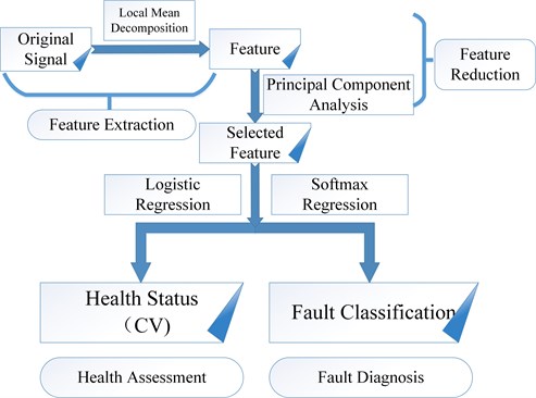
The proposed method has two steps: the first step involves the feature extraction and selection that determines the appropriate features for health assessment and fault classification, as well as reduces the search space for fast computation; the second step involves health assessment based on the LR model and fault classification based on the softmax regression model. The process of the method is summarized in Fig. 1.
Fig. 1Process of the proposed method
2.2. Feature extraction by using local mean decomposition
The LMD scheme involves separating a frequency-modulated signal from an amplitude-modulated envelope signal. The process of the separation includes smoothing the original signal, subtracting the smoothed signal from the original signal, and using an envelope estimate to amplitude demodulate the result. By using moving averaging weighted by the time lapse between the successive extrema of the original signal, the envelope estimate and smoothed version of the original signal are both obtained. The procedure will not stop until a frequency-modulated signal with a flat envelope is obtained. A final envelope is formed by multiplying the corresponding envelope estimates together. This envelope is then multiplied by the frequency-modulated signal to form a product function. The whole process is repeated on the resulting signal to acquire a second product function with an associated envelope and instantaneous frequency. When the remaining signal contains no oscillations, the decomposition is finally completed.
For any signal x(t), the steps of LMD are given in the following:
First, the identification of all local extrema values ni should be conducted. The ith mean value mi of each two successive local extrema values is calculated as follows:
The local means can be connected with straight lines between successive extrema. To obtain the corresponding smoothly varying continuous local mean function, the local means are smoothed by moving averaging.
Then, the envelope estimate ai is calculated by using the local extremum ni:
The successive envelope estimates ai can also be connected with straight lines. In the same manner, the local magnitude of each half-wave oscillation is smoothed to the same degree as the local means.
The next step is to separate the local mean function m11(t) from the original signal x(t):
h11(t) is demodulated by dividing it by the envelope estimate function a11(t):
where a11(t) is a pure amplitude-modulated signal; thus, the envelope estimate function is a12(t)=1. If s11(t) does not meet the criteria, the iterative process above will be repeated with s11(t) as the original data until a pure amplitude-modulated signal s1n(t) is obtained. Thus, -1≤s1n(t)≤1 and a1(n+1)(t)=1. The following is then obtained:
where:
The termination condition of the iterative process is expressed as follows:
The envelope function a1(t), namely the instantaneous amplitude function, is obtained by multiplying all the envelope estimate function achieved in the iterative process:
The first product function of the original signal is obtained by multiplying the envelope signal a1(t) by the pure frequency-modulated signal s1n(t):
where PF1(t) has the highest frequency component of the original signal, and it is an amplitude- and frequency-modulated signals with simple components. The instantaneous amplitude function of the original signal is the envelope signal a1(t). The instantaneous frequency function f1(t) is expressed as follows:
A new signal u1(t) is obtained by separating the first product function PF1(t) from the original signal x(t), and the whole process is repeated for k times with u1(t) as the original signal until uk(t) is a constant or contains no oscillations:
The original signal can then be represented as follows:
The LMD is complete because the original signal is reconstructed [4].
The feature vector of the hydraulic pump vibration signals contains 12 components that are calculated from the 4 product functions obtained from the LMD. The feature vector T is expressed as follows:
where g11,g21,…, gm1 and g21,g22,…, gm2 are the skewness coefficients and kurtosis coefficients of the product functions, which are defined as follows:
The energy value of each product function is given by the following:
For the convenience of data processing and analysis, the energy vector is normalized as follows [5]:
2.3. Feature reduction based on multidimensional scaling
Multidimensional scaling (MDS) is a means of visualizing the level of similarity of individual dataset cases. MDS aims to place each feature in N-dimensional space such that the between-object distances are preserved as well as possible. Each feature is then assigned coordinates in each of the N dimensions.
The data to be analyzed is a collection of I features wherein a distance function is defined as δi,j≔distance between th and th features.
These distances are the entries of the dissimilarity matrix:
The goal of MDS is finding vectors that , ,…, such that for all , 1,…, under the condition that is given, where is a vector norm. The norm of MDS can be the Euclidean distance and a metric or arbitrary distance function in a broader sense.
Thus, MDS attempts to find an embedding from the features into ( indicates the set of real numbers, and refers to the Cartesian product of copies of , which is an -dimensional vector space over the field of real numbers) such that distances are preserved. If the dimension is chosen to be two or three, the vectors can be plotted to obtain a visualization of the similarities between the objects. The vectors are not unique. By using the Euclidean distance, the vectors may be arbitrarily translated, rotated, and reflected because these transformations do not change the pairwise distances .
Various approaches can be used to determine the vectors . MDS is normally formulated as an optimization problem, where , ,…, is a minimizer of some cost function, e.g.:
A solution may then be found by using numerical optimization techniques. For the chosen cost functions, minimizers can be stated analytically in terms of matrix eigendecompositions [6-8].
2.4. Logistic regression method
The machine condition description from daily maintenance records/logs is a dichotomous problem (either normal or failed) that can be represented by using a LR function [1]. The goal of LR is to find the best fitting model to describe the relationship between the categorical characteristic of a dependent variable (the probability of an event, ranging from zero to one) and a set of independent variables. The logistic function is expressed as follows:
The logistic model is defined as follows:
where is a linear combination of independent variables , ,…, .
The pre-condition for determining is determining parameters and ,…, in advance. Given that the dichotomous dependent variable hinders the estimation by ordinary least squares, estimation in LR chooses parameters of and ,…, by using the maximum likelihood method rather than choosing parameters that minimize the sum of squared errors [9-10]. Then, the probability of failure for each input vector can be calculated according to Eq. (20).
2.5. Softmax regression method
The softmax regression model generalizes LR to classification problems that can be used in multi-class classification problems where classes are mutually exclusive. A training set of softmax regression is generated as of labeled examples, where the input features are . As opposed to binary classification, the label can be different values instead of only two values. Thus, in the training set . For example, for a hydraulic pump with two different types of fault, the will be three when taking the normal state into consideration.
The purpose of softmax regression is to estimate the probability of the class label that is addressing each of the different possible values. Thus, for a test input , the probability that for each value of 1,…, is estimated by hypothesis. The hypothesis outputs a dimensional vector (whose elements sum to 1) and provides estimated probabilities. The hypothesis is given by the following:
where , ,…, are the parameters of the softmax regression model. Normalized by , the hypothesis for equals to one.
For convenience, is used to denote all the parameters of the model and is usually obtained by stacking , ,…, in rows to form a -by-(1) matrix:
The cost function of the softmax regression is expressed as follows:
In the equation above, is the indicator function such that 1{a true statement} = 1 and 1{a false statement} = 0. An iterative optimization algorithm such as a gradient descent or L-BFGS is used to solve for the minimum of . The gradient is obtained by taking derivatives:
where the th element of the vector is being the partial derivative of with respect to the th element of.
Softmax regression has a redundant set of parameters. Thus, subtracting some fixed vector from the parameter vectors does not change the result of the class label probabilities estimated by the hypothesis. In this way, the softmax model is over parameterized, i.e., for any hypothesis that may fit the data, multiple parameter settings exist that give rise to exactly the same hypothesis function mapping from inputs to the predictions. Therefore, the cost function is modified by adding a weight decay term, which penalizes large values of the parameters. The cost function is now expressed as follows:
With the weight decay term (for any ), the cost function is now strictly convex and is guaranteed to have a unique solution. To apply an optimization algorithm, the derivative of the new definition of is needed. The new definition is expressed as follows:
A working implementation of softmax regression will be obtained by minimizing with respect to [10-12].
3. Case study
The proposed method was applied to evaluate the health condition of a hydraulic pump (Fig. 2). To classify the possible root cause, fault analysis was performed.
Fig. 2Experimental test plunger pump rig
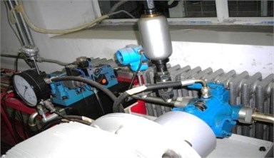
In this study, two commonly occurring faults in the hydraulic pump were injected: slipper loosing and valve plate wear. The vibration signals of the hydraulic pump were acquired from the end face with a stabilized motor speed of 528 rpm and 1000 Hz sampling rate. A total of 12 samples were acquired under the normal condition, and four samples were obtained for each of the two fault states.
3.1. Feature extraction and reduction
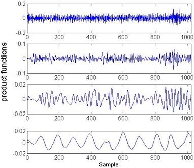
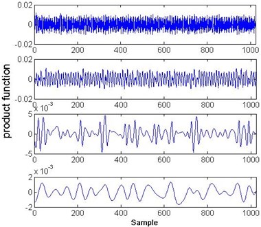
First, each vibration signal was processed by LMD to acquire the product functions. Fig. 3(a) shows the result of the LMD of the normal condition signal, and Fig. 3(b) shows the result of the LMD of the signal under slipper loosing condition. Second, the skewness coefficients, kurtosis coefficients, and normalized energy values of the product functions was calculated to form the feature vector. MDS was then used to determine a subset of feature components. In this case, a three-dimensional feature vector was finally used for the health assessment and fault mode classification.
Fig. 3LMD results of normal and slipper loosing conditions
a)
b)
3.2. Training of logistic regression and softmax regression models training
3.2.1. Logistic regression model training for health assessment
The training data contains 240 sets of data, including 80 sets of normal condition ( 0) data and 160 sets of fault data ( 1). The parameters and ,…, estimated by the maximum likelihood method was eventually used to obtain the model for performance assessment as LR.
3.2.2. Softmax regression model training for fault classification
Two fault modes of the hydraulic pump were considered, including valve plate wearing and slipper loosing. Two sets of hydraulic pump vibration data (one set for each fault mode of the hydraulic pump) were used for training the fault diagnose model based on softmax regression.
Fault mode 1 (valve plate wear): 200 sets of valve plate wearing data versus 200 sets of normal data were used to train the fault classification model for fault model 1.
Fault mode 2 (slipper loosing): 200 sets of slipper loosing data versus 200 sets of normal data were used to train the fault classification model for fault model 2.
To obtain the parameters (, ,…, )of the softmax regression fault classification model, the gradient descent method was used.
3.3. Validation of the proposed method
For each fault mode, one set data of the hydraulic pump were used for validation.
Set 1 (fault mode 1): 40 sets of data under normal condition versus 80 sets of valve plate wear data.
Set 2 (fault mode 2): 40 sets of data under normal condition versus 80 sets of slipper loosing data.
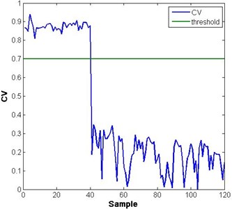
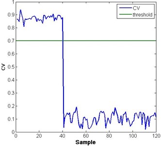
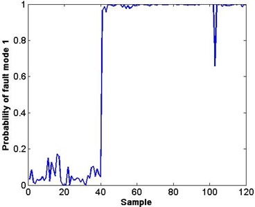
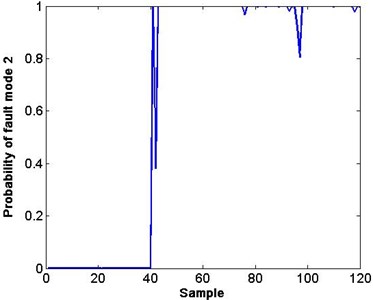
The confidence value (CV) was defined as , where is the probability of failure. When the pump is running normally, CV is close to one. However when the pump is going to fail, the CV will approach zero correspondingly. In the course of a decreasing CV, as long as the value is less than 0.7 (a preset threshold), the fault mode classification model is triggered to input the features into the softmax regression model to classify each fault. Fig. 4(a) and (b) shows the result of the overall health assessment of the two sets of vibration data of the hydraulic pump by using the LR model. Fig. 5(a) and (b) shows the different fault mode probabilities obtained from LR 2 and LR 3.
Fig. 4Health assessment result of two fault modes
a)
b)
Fig. 5Probability of fault modes 1 and 2
a)
b)
In Fig. 4, both faults can be detected from the decreasing CV. However, clarifying the difference and reason of this decrease is still difficult. To solve this problem, the softmax regression classification module is used. As long as the CV falls below 0.7, the probability of the fault modes will be calculated by inputting the corresponding features into the trained softmax regression model. In Fig. 5(a) and (b), the probability of fault 1 (valve plate wear) and fault 2 (slipper loosing) is high from the 40th sample. The small probability points of the corresponding fault are shown in Fig. 5.
A softmax regression classifier is more convenient for hydraulic pump fault classification than two separate LR binary classifiers. Given that the fault modes mentioned in this study are mutually exclusive from each other, the softmax regression model will be more appropriate than the aforementioned modes.
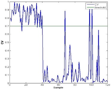
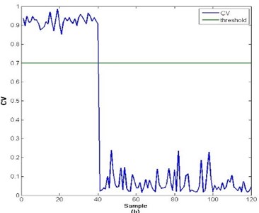
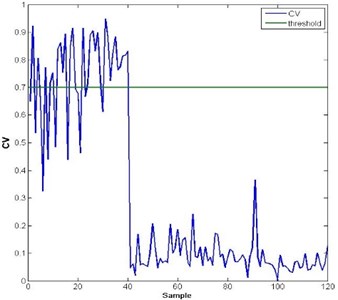
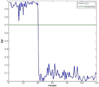
The ability of the methodologies’ anti-noise capacity is tested by adding additive noise to the original signals. The selected additive noise in the test is Gaussian white noise, and the SNR is set from 1 dB to 90 dB at interval of 1 dB. In the anti-noise ability test of health assessment, we find that as long as the SNR is above 30 dB, the health assessment model is able to function well as in the standard fault scenarios. Fig. 6 and Fig. 7 show the test result with noise added to the origin signals in health assessment. Fig. 6(a) is the health assessment result when SNR is under 30 dB and Fig. 6(b) is the health assessment result when SNR is above 30 dB of fault mode 1. Similarly Fig. 7(a) is the health assessment result when SNR is under 30 dB and Fig. 7(b) is the health assessment result when SNR is above 30 dB of fault mode 2. According to the test result, when SNR is above 25 dB, the health assessment model functions as well as in the standard scenarios.
Fig. 6Test result of health assessment with additive noise of fault mode 1
a)
b)
Fig. 7Test result of health assessment with additive noise of fault mode 2
a)
b)
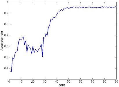
The result of the test for fault mode classification is shown in Fig. 8. When SNR increases from 1 dB to 50 dB, the accuracy rates changes from around 40 % to 95 % with a general upward trend. When SNR is above 50 dB, softmax regression model can classify the fault modes of the pump effectively with an accuracy rate over 95 %. For every SNR value, the value of -coordinate in Fig. 1 is the average accuracy rate of 10 values.
Fig. 8Test result of fault classification accuracy rates with additive noise
4. Conclusion
The health assessment and fault classification of a hydraulic pump based on LR and softmax regression was performed in this study. LMD combined with MDS can obtain appropriate features from non-stationary vibration signals. LR combined with the maximum likelihood estimation is an effective and efficient tool for health assessment, whereas the softmax regression model is an effective tool for dynamic fault classification. The method not only processes non-stationary signals but also stationary signals. Thus, the method can be generalized and applied to the other vibration signals of pumps. However, additional fault modes should be taken into consideration to achieve a better performance on hydraulic pump health assessment and fault classification.
References
-
Frank P. M. Fault diagnosis in dynamic systems using analytical and knowledge-based redundancy – a survey and some new results. Automatica, Vol. 26, 1990, p. 459-474.
-
Gertler J. J. Survey of model-based failure detection and isolation in complex plants. IEEE Control Systems Magazine, Vol. 8, 1988, p. 3-11.
-
Wang Shaoping, Zhongkui Yuan, Guangqin Yang Study on fault diagnosis of data fusion in hydraulic pump. Zhongguo Jixie Gongcheng (Chinese Journal of Mechanical Engineering), Vol. 16, Issue 4, 2005, p. 327-331.
-
Smith J. S. The local mean decomposition and its application to EEG perception data. Journal of the Royal Society Interface, Vol. 2, Issue 5, p. 443-454.
-
Cheng J. S., Shi M. L., Yang Y. Roller bearing fault diagnosis method based on LMD and neural network. Journal of Vibration and Shock, Vol. 29, Issue 8, p. 141-144.
-
de Leeuw J., Heiser W. Theory of Multidimensional Scaling. Handbook of Statistics, Vol. 2, 1982, p. 285-316.
-
Flexer A. Limitations of self-organizing maps for vector quantization and multidimensional. Advances in Neural Information Processing Systems 9: Proceedings of the 1996 Conference, Vol. 9, 1997, p. 445.
-
Kruskal J. B. Multidimensional scaling by optimizing goodness of fit to a nonmetric hypothesis. Psychometrika, Vol. 29, Issue 1, 1964, p. 1-27.
-
Hosmer D. W., Lemeshow S., Sturdivant R. X. Introduction to the Logistic Regression Mode. John Wiley and Sons, Inc., 2000.
-
Yan J., Lee J. J. Degradation assessment and fault modes classification using logistic regression. Journal of Manufacturing Science and Engineering, Vol. 127, Issue 4, 2004, p. 912-914.
-
Gimpel K., Smith N. A. Softmax-margin CRFs: training log-linear models with cost functions. Human Language Technologies: The 2010 Annual Conference of the North American Chapter of the Association for Computational Linguistics, Association for Computational Linguistics, 2010, p. 733-736.
-
Memisevic R., Zach C., Pollefeys M., et al. Gated softmax classification. Advances in Neural Information Processing Systems, 2010, p. 1603-1611.
About this article
This research was supported by the Technology Foundation Program of National Defense (Grant No. Z132013B002).
