Research on fault diagnosis of hydraulic pump using convolutional neural network

2.1. The theory of CNN

CNN is a feed-forward neural network, and it extracts topology from a two-dimensional image through back-propagation algorithm to optimize the network, in order to compute the nodes in the network [15]. The introduction of one-dimensional CNN network is followed.

2.1.1. The structure of CNN

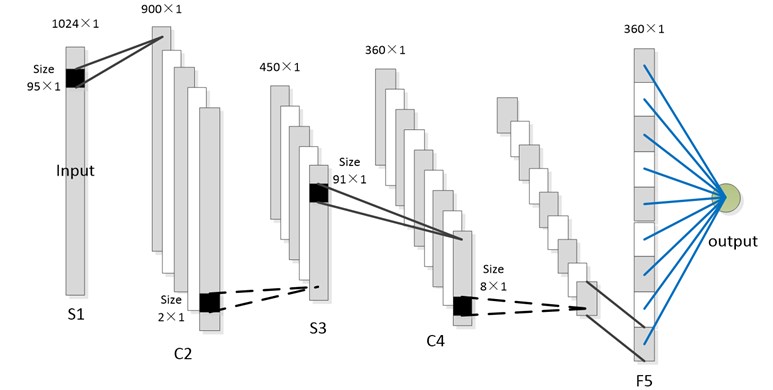
Fig. 1 is a typical 6 layer CNN, including input layer, output layer, convolution layer, subsampling layer and full connection layer. One dimensional signal is input into input layer, through repeated subsampling layer (S), convolution layer (C) and the last full connection layer (F), finally, the output layer gives the label.

Both the S and C have several feature maps, and each map connects with the former layer. At a convolution layer, the previous layer’s feature maps are convolved with learnable kernels and input a activation function to constitute the output feature map.

In Fig. 1, the convolution layer are C2 and C4, and followed by S. Each feature map in a convolution layer may connect to several feature maps in previous layer. The input signal is ${\mathbf{x}}_j^l\in {\mathbb{R}}^{n\times 1}$, indicates the number of layer, $j$ is number. The convolution kernel is a column vector ${\mathbf{k}}_{ij}^l$. $i$ is the number of feature map in convolution layer. The convolution layer can be represented as:

1

${\mathbf{x}}_j^l=f\left({\mathbf{z}}^l\right),\mathrm{}\mathrm{}\mathrm{}\mathrm{}\mathrm{}{\mathbf{z}}^l=\sum _{i\in M_j}{\mathbf{x}}_i^{l-1}\mathrm{*}{\mathbf{k}}_{ij}^l+b_j^l.$

Fig. 1One dimension CNN

Each feature map corresponds several convolution kernels. $M_j$ is a selection of input feature map, here the full connection is chosen, thus each convolution layer has a bias. The main task of convolution layer is to translate former layer in different perspective for constructing model. The convolution layer is usually followed by a subsampling layer:

2

$x_j^l=down\left(x_i^{l-1}\right)=\mathrm{m}\mathrm{a}\mathrm{x}{x}_i^{l-1}\left(u{}_1{}^{},u_2\right),$

where $\left(u{}_1{}^{},u_2\right)$ represents the pooling scale in previous layer. The purpose of pooling is to reduce resolution and improve computational efficiency, at the same time to enhance the robustness to scaling and distortion. Many experiments have shown this simple way is very effective.

2.2. Computing CNN

CNN needs to be computed after, and if its parameters are updated as traditional neural network, each connection will have a parameter which should to be learned. In this condition, the parameters will be too numerous to update. The weight sharing adopted by CNN can greatly reduce the free parameters through sharing the same weight in the same feature map, which can detect the different transform from different perspective using the same kernel.

As shown in Fig. 1, the neuron in layer C is calculated by the area connected to it. Similarly, the neuron in layer S should be computed by the local field connected to it in previous layer, in this way, the feature map is constructed. In CNN, any neuron in each layer is computed through the local field in previous layer connected to it after a output activation function. Finally, the output layer outputs result, namely the condition of the pump is recognized.

In CNN, weight update is based on the back-propagation algorithm, the update of weight $w$ from iteration $t$ to $t+1$ is as followed:

where $\eta$ is learning rate, $x\left(t\right)$ is the input of neurons. $\delta \left(t\right)$ is the error term of the neuron, the error term $\delta \left(t\right)$ have different expression for output neurons and hidden neurons, and it is usually computed by gradient descent method. References [11, 16, 17] give the details of weight update in CNN.

2.3. Weighted sum

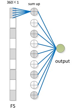
As showed in proposed CNN structure, in the last layer namely the full connection layer, the neurons in the same feature map still contains relative position information, thus the translation cannot be completely eliminated. To overcome this challenge, a weighted sum strategy is added to further improve the shift-invariance of CNN. As shown in Fig. 2, a new layer is inserted between the full connection layer and output layer. This new layer sums up the neurons in the same feature map in order to remove the influence of relative position information. This algorithm reduces the neurons used for recognition and also decreases the complexity of network, and it is easy to use and understand. Although it is simple, it indeed effectively enhances the robustness of CNN to translation, and lastly enhances the recognition effect.

Fig. 2Weighted sum

2.4. Diagnosis procedure

The traditional fault recognition model is as shown in Fig. 3. Firstly, complex pre-process is applied to filter the noise and reduce the influence of variable conditions. Then is feature extraction and selection which should be on the foundation of adequate professional knowledge. The operator’s quality is highly demanding in this step, and whether the extracted feature is good enough mainly determines the accuracy of fault diagnosis later. Finally, a classifier is used for fault recognition, and the diagnostic result is acquired. The primary improvement of CNN classification model is that it directly learns the signals measured from sensor without other processing, as displayed in Fig. 4, which considerably reduces the steps. This new model relies on the robustness of CNN to interference, distortion, scaling. It uses CNN to construct the model by the data itself, and automatically finds the internal structures of original data.

Fig. 3Traditional classification model

Fig. 4CNN classification model

3.1. Introduction of experiment

MCY14-1B axial piston pump is small, light, compact and convenient for maintenance, and it is suitable for the machinery in ship, aviation, mining and so on. The type of the hydraulic pump in this experiment is 25MCY14-1B, and it has 7 plunger. Its nominal flow-rate is 25 ml/r, and the nominal pressure of 31.5 MPa.

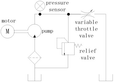
The hydraulic pump was driven by a three-phase asynchronous motor of 5.5 kW, and the motor was controlled by a frequency converter. The outlet of the hydraulic pump connected a throttle valve and a relief valve, and finally linked to the tank. In this experiment, the load was imposed by the throttle valve, and relief valve kept safety, with the maximum relief pressure was 16 MPa. The vibration signal of the hydraulic pump was measured for fault diagnosis, and its sampling frequency is 10 kHz. The test rig is as shown in Fig. 5, and the schematic diagram is shown in Fig. 6.

Fig. 5Test rig

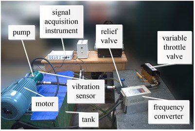
Fig. 6The schematic diagram of the test system

The axial piston pump’s pressure is high and its speed is fast, so it is prone to failure. According to statistics [3], the easiest failure components include cylinder, valve plate, piston, rolling and spring, etc. Six kinds of faults were simulated in this paper, as shown in Fig. 7.

Fault 1: cylinder wear, here cylinder was equivalent to an inner ring of bearing, and the fault was cut as depth of 0.5 mm, width of 0.2 mm.

Fault 2: valve plate wear, the faulty valve plate was chosen in a faulty pump.

Fault 3: roller wear, the fault was cut as depth of 0.5 mm, width of 0.3 mm.

Fault 4: loose slipper, the gap of piston was 0.25 mm.

Fault 5: sliding boot wear, its wear loss is about 0.25 mm compared to normal one.

Fault 6: spring wear, the wear loss of spring was about 0.25 mm.

Fig. 7The faults setting

The pump speed was 600 r/min, 900 r/min and 1200 r/min respectively in the experiment, so the rotating frequency was 15 Hz at the speed of 900 r/min, and the fundamental frequency of pressure pulsation was 7×15 = 105 Hz. The diameter of the outer ring of the bearing is 107.5 mm, and the diameter of inner ring namely the cylinder is 96.5 mm. The number of rollers is 22, and its diameter is 11 mm. The outer ring is fixed when pump is working. Therefore, the characteristic frequency of outer ring is about 148.12 Hz, the roller is about 146.45 Hz, and the cylinder (or inner) is about 181.89 Hz.

Fig. 8Vibration signal in time domain and frequency domain of each condition

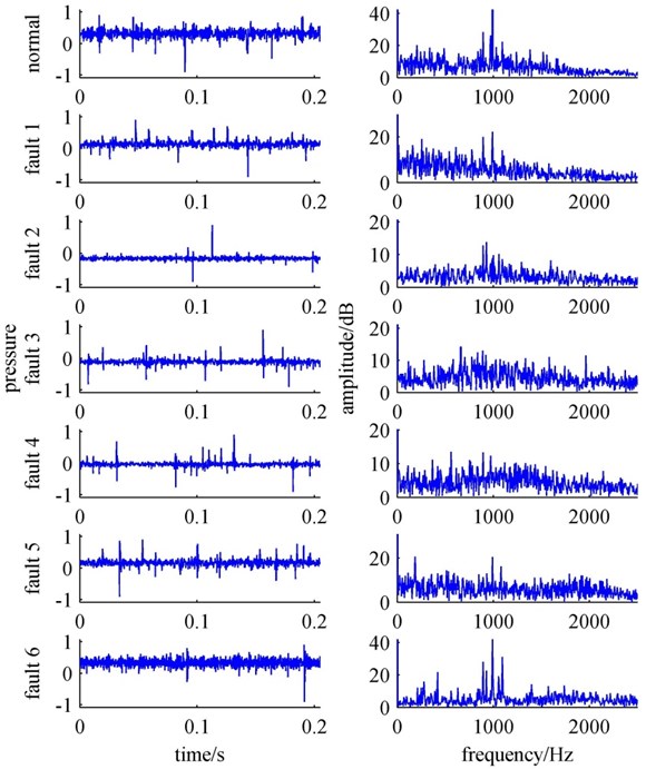
The hydraulic pump which is complex has many vibration sources. The faulty pump not only changes at characteristics frequency, but also at rotating frequency and natural frequency. Therefore, if we use the characteristic frequency for fault recognition, it will be not only difficult to identify the pump condition, but also losses some potential information. Especially for slight failure with heavy disturbance, it adds more difficulties. Fig. 8 is the vibration signal in time domain and frequency domain of each condition. Although it was under lab experiment, the surrounding noises as well as electromagnetic interference were not removed, thus it was more close to real fault diagnosis. The electromagnetic interference is obvious in each vibration signals. The vibration signal of hydraulic pump is complicated and contains lots of noises. It is nonlinear, leading to difficulties to extract the features which can reflects the status information of the hydraulic pump. From those we can know that, the traditional diagnostic approaches are not easy to diagnose conveniently. Therefore, the following researched how to apply CNN for correct and convenient fault diagnosis of hydraulic pump.

3.2. Fault diagnosis and comparison under the stable operating condition

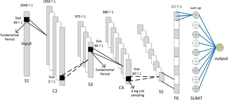
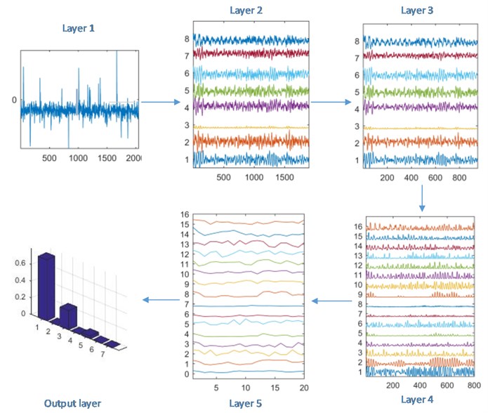
This section employed proposed method to diagnose the hydraulic pump on the stable speed of 900 r/m. For simple network setting, according to the mechanism of hydraulic pump, an convenient network setting method based on experience was put forward. The CNN in this experiment has 7 layers, as shown in Fig. 9. The first layer is input layer, the 6th layer is full connection layer, and the 7th is the weighted sum layer. The 2th and 4th layer are both convolution layers, and the size of a kernel approximately corresponds a fundamental frequency, here it is termed as basic period. Because hydraulic pump is a rotating machinery, the vibration waveforms in a basic period under different conditions have significant differences, and 2th layer is used to extract and recognize these differences.

After the subsampled with scale of 3th in third layer, although the convolution kernel scale still corresponds to a basic period in layer 4, it corresponds to two basic period of the input in actual. Therefore, this kernel can also detect the variation of basic period caused by condition changes. The 2th layer was used to extract local information, and the 4th layer was to extract more comprehensive information. This network designing scheme is a good and convenient one validated in experiments, and it also effects for rotating machinery.

Layer 3 and layer 5 are both subsampling layer, the subsampling scale in layer 5 can be a larger one. In this way, it can not only reduce the number of network nodes, but also suppresses the influence of noises and enhances the robustness. At the CNN of this experiment, the 2th layer has 8 feature maps, and the 4th has 16 ones. The scale of each feature map is as displayed in Fig. 9. The activation function is a tanh-function, and output function is a softmax classifier.

Fig. 9The CNN structure in experiment

In order to completely verify the fault diagnosis performance by CNN, it was also compared with DBN, support vector machine (SVM) and BP neural network. However, these three algorithms cannot keep shift-invariance, so all the samples were converted to the spectrum for fault recognition. Each class of training set had 100 samples, and each class of test set had 300 samples.

The result is represented in Fig. 10, all the results are the average for ten times of experiments. The accuracy rate of CNN is the highest. Apart from accuracy rate, only CNN directly applies the original data without any additional steps, whereas other methods need attached pre-processing such as time-frequency transform and de-noising. Overall, all of these algorithms work well in this experiment, and the worst one has the accuracy rate above 95 %. This is because the speed was stable, so the training samples are similar to the test samples, so even simple algorithms can do this diagnosis. However, the speed of the pump in application cannot always works in such stable condition, so the fault diagnosis of variable speed has more engineering significance.

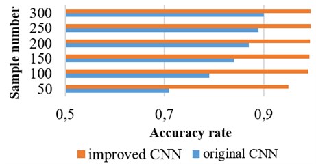
Furthermore, the original CNN without weighted sum was also tested, to verify the improved strategies. The training samples are chosen as 50, 100, 150, 200, 250, 300, respectively. The result is as shown in Figure 11. The CNN proposed in this paper is superior to original CNN. As the training samples become more, the original CNN performs better. Because the features extracted by the original CNN still have certain position information, when the training samples are few, it is difficult to distinct different condition of hydraulic pump. However, as the number of training samples grows, the shortage will be covered in a certain degree. The improved CNN is invariant to period features, thus it works well although the training samples are few. This experiment further demonstrates that the weighted sum is proper for the hydraulic pump.

Fig. 10The accuracy rate for stable working condition

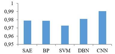
Fig. 11The accuracy rate of original CNN and improved CNN

3.3. Fault diagnosis and comparison under the condition of variable speed

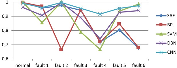
This experiment was the fault diagnosis of hydraulic pump with variable speed, and other algorithms were also compared. Here the training samples were taken from the speed of 600 r/m and 1200 r/m, and the test samples are from 600 r/m, 900 r/m and 1200 r/m. The recognition result is shown in Fig. 12, and Fig. 13 is the accuracy rate of each state.

Fig. 12The accuracy rate for variable speed

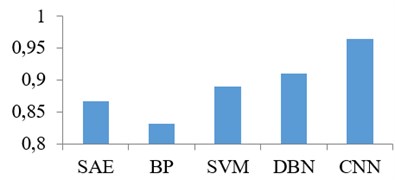
It is known from the fault recognition result, the accuracy rate of CNN is the highest, and the worst one is above 90 %. The accuracy rate of CNN is close to the accuracy rate of stable speed, yet the other methods degrade sharply. Due to excellent robustness to scaling, CNN is not sensitive to the variation of speed, so that it is appropriate to the real fault diagnosis of hydraulic pump in application. When the speed varies, the frequency spectrum of vibration signal will changes correspondingly, so the other machine learning algorithms were influenced. On the other hand, if the other machine learning algorithms directly used the time domain signal for fault recognition, the performance will be worse. Although DBN is one of deep learning algorithm, it is weak robust to scale. Thus, its fault recognition is not good enough, and its accuracy is the second. The shallow learning method such as SVM and BP neural network perform worse because they are short of the ability to learn from complex data. Due to the actual significance of fault diagnosis with variable speed, this experiment illustrates that the proposed CNN algorithm is applicable to the fault diagnosis of hydraulic pump even the speed is variable.

Fig. 13The accuracy rate of each state

3.4. The fault separation of hydraulic pump

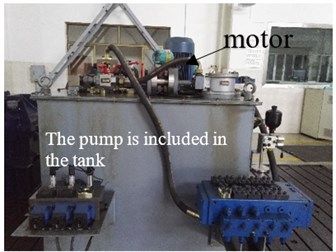
Fig. 14 is a hydraulic pressure station, it supplies a driven system. In August 2015, the strength of driving system was too weak to work, and the faulty place is unknown. Possible part is pump, valve or actuator. Firstly, the pump was tested, and it was installed on the test rig to measure the vibration signal. The parameters in this experiment were the same as section 3.3, only the test speed was set as 900 rpm. Ten samples were tested, and 9 samples showed normal and one was as sliding boot wear. The procedure of one normal sample put in improved CNN is displayed in Fig. 15. Therefore, the diagnosis of normal is reliable, then it is found that the actuator was failure.

Fig. 14Hydraulic pressure station

In April 2016, the output power of system was insufficient, and the noise of the hydraulic pump increased when the pressure was high. The hydraulic pump was measured another time and ten samples were measured. Eight samples showed loose slipper, and one as roller wear, another one as valve plate wear. Then the hydraulic pump was disassembled and showed loose slipper. After the replacement of all the plungers, the system worked well again.

The application showed that this scheme can guide the fault diagnosis of hydraulic pump to a certain extent. In the future, the hydraulic pump will be tested under working without disassembling, and the real-time monitoring of the fault diagnosis will also be tried.

Fig. 15Hydraulic pressure station