An investigation into frequency resolution estimation model for impact signal analysis by using Hilbert spectrum and condition classification for marine diesel engine

Li, Hongkun; Zhang, Xiaowen; He, Delu; Zhou, Peilin

Journal of Vibroengineering

Browse Journal

Submit article

Published: 30 September 2014

Check for updates

An investigation into frequency resolution estimation model for impact signal analysis by using Hilbert spectrum and condition classification for marine diesel engine

Hongkun Li¹

Xiaowen Zhang²

Delu He³

Peilin Zhou⁴

^{1, 2, 3}School of Mechanical Engineering, Dalian University of Technology, Dalian, 116024, China

⁴Department of Naval Architecture, Ocean and Marine Engineering, University of Strathclyde, Glasgow, G4, United Kingdom

Corresponding Author:

Hongkun Li

Cite the article Download PDF

Downloads 1164

Abstract

In this paper, frequency resolution determination method is investigated according to Hilbert spectrum performance for impact signal analysis. A new constructed performance estimation model for the best frequency resolution is put forward in this research for the impact signal pattern recognition. Different parameters in the time-frequency distribution by using Hilbert spectrum are considered in this estimation model for the best frequency resolution determination. To verify the effectiveness of this estimation model, numerical simulation is used for Hilbert spectrum construction analysis. At the same time, different marine diesel engine working condition signals analysis are also used to illustrate the methodology developed in this research and verify the effectiveness. It can be concluded that this method can contribute the development for impact signal analysis by using Hilbert spectrum.

1. Introduction

Nowadays, working machine’s condition monitoring and fault diagnosis become more and more important since fault condition will affect normal production process and even lead to serious catastrophe of the machine. Fault diagnosis and early detection are very essential to prevent larger failure. At the same time, it is convenient for condition maintenance for slight fault. Vibration signal analysis has been broadly used for machine condition monitoring and classification. When a machine is in fault condition, its vibration signal is usually full of nonstationary and nonlinear characteristics. At the same time, there are lots for noise and other source interference for practical signal analysis. Thus, weak fault feature extraction of key machine is one of the key questions for early fault diagnosis [1].

Time frequency distribution (TFD) analysis has been applied in different area for instantaneous impact signal analysis (IISA) because it contains both time and frequency domain information. The impact information can be easily determined by using TFD compared with time or frequency domain analysis. Therefore, it is convenient to feature extraction and condition classification for nonstaitonary and nonlinear signal analysis. But the accuracy of classification also depends on the TFD concentration. Nowadays, reassignment method has been applied on quadratic TFD analysis for better feature extraction and condition classification [2]. Hilbert spectrum analysis (HSA) was introduced by Norden Huang in 1998 [3]. It is a self-adaptive decomposition process and developed from instantaneous frequency (IF). Since then, it has been broadly investigated by many researchers, such as vibration signal analysis [4], climate anomalies analysis [5], seismic signal analysis [6]. Original signal can be decomposed into several intrinsic mode functions (IMFs) according to empirical mode decomposition (EMD). A new calculation method named ensemble empirical mode decomposition (EEMD) is put forward by Zhaohua Wu and Norden Huang [7]. It is also the development for EMD. Hilbert spectrum (HS) can be calculated by using Hilbert transform for IMFs obtained by EEMD. HS can be expressed in two-dimension or three-dimension plot. HS is more suitable for non-stationary and nonlinear signal analysis as it is developed from IF. But there are several key questions to be solved for this developing method, such as EMD method for further improvement, theory basis for the decomposition, frequency resolution (FR) of Hilbert spectrum, and so on [3, 7, 8]. Among these questions, FR for HS is seldom investigated by researchers. FR can be selected randomly as there is not any clear definition which on is the best determination method. It is just according to visual inspection. FR of HS is different from traditional method such as short time Fourier transform, Wigner-Ville distribution, wavelet analysis, etc. [8]. It also has direct effect on HS for signal analysis. Although many researchers pay more attention for this area, this is not a clear definition to estimate the performance of FR [8]. Therefore, it is very necessary to construct an estimation model for the best FR determination.

It is well known that performance for TFDs are commonly compared according to energy concentration and accuracy for signal expression. For a TFD $ρ (t, f)$ in practical signal analysis, a more appropriate interpretation would be as a measure of energy flow through the spectral window $(f - Δ f / 2, f + Δ f / 2)$ during time interval $(t - Δ t / 2, t + Δ t / 2)$ . The energy localized in the time-frequency region $(Δ t, Δ f)$ is given by [9]:

1

E_{Δ t, Δ f} = \int_{t - Δ t / 2}^{t + Δ t / 2} \int_{f - Δ f / 2}^{f - Δ f / 2} ρ (t, f) d f d t .

It is clear that high FR has good performance on feature extraction and condition classification if the time resolution is determined according to Eq. (1). Within a frequency analysis range, the bigger is frequency number, the smaller is FR. It will give more information for IF. But it doesn’t mean that the smaller is FR, the better is HS demonstration. There will be the best FR by using TFD [10]. Thus, it is very important to determine the best FR for HS although its construction process is different compared with quadratic TFD. Fig. 1 is the sketch map for different FR corresponding to different HS. When the frequency cell number is very small, the energy will be concentrated as some small energy belonging to one time-frequency cell shown in Fig. 1(a). Thus, it is very difficult to separate small frequency variation in TFD plane. With frequency cells increasing, FR $Δ f$ will decrease shown as Fig. 1(b). It will give more information for IF. At the same time, the energy will disperse. When $Δ f$ is very low, the energy of every time-frequency cell will be also small. It affects the analysis result by using HS because the energy is very dispersive. Thus, the frequency cells should not be very small or large. There should be the best frequency cell to construct HS. Thus, FR estimation method is very urgent needed to improve HS performance on signal analysis.

Fig. 1Sketch map for different FR effect on HS

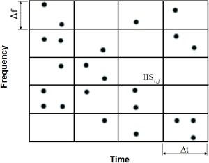
a) Low frequency cells

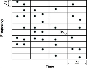
b) High frequency cells

In this research, a new model is constructed to estimate the performance of FR for HSA in detail. According to the simulation signal and practical vibration signal analysis, it can be concluded that the estimation model is effective for HS construction and feature extraction. The rest of the paper is organized as following. In Section 2, the theory of HS analysis is introduced. Estimation model and simulation signal analysis are presented in Section 3. Practical diesel engine vibration signal analysis according to the estimation model is demonstrated in Section 4. Some conclusions are finally drawn in Section 5.

2. Hilbert spectrum

To get a meaningful Hilbert spectrum, a new signal decomposition was introduced by Huang named as empirical mode decomposition [3, 4]. According to EMD, original data is decomposed to $n$ intrinsic mode components $C_{i} (t)$ and a residual component $r_{n}$ as Eq. (2). Nowadays, EEMD is also greatly applied in signal analysis because it is a self-adaptive decomposition process. In this research, EEMD is used to decompose signal into IMFs according reference [7]:

2

X (t) = \sum_{j = 1}^{n} C_{j} (t) + r (t) .

After getting each IMF component, Eq. (3) can be obtained. It gives both the amplitude and the frequency of the real part (RP) for each component as a function of time:

3

X (t) = R P \sum_{j = 1}^{n} a_{j} (t) e^{i θ_{j} (t)} = R P \sum_{j = 1}^{n} a_{j} (t) e^{i \int ω_{j} (t) t} .

Both the amplitude and the IF can be represented in a three-dimensional plot, in which the amplitude can be contoured on a time-frequency plane. The TFD of the amplitude is expressed by the Hilbert spectrum, as shown in Eq. (4):

4

H S (ω, t) = R P \sum_{j = 1}^{n} a_{j} (t) e^{i \int ω_{j} (t) t} .

HS is different from others quadratic TFDs. HS developed from instantaneous frequency, there is not any negative frequency. It is the main difference between HS and quadratic TFD. Therefore, it is more suitable for nonstationary and nonlinear signal analysis. Huang has given a suggestion on how to determine the best frequency resolution. The maximum number of the frequency cells, $N$ , of the HS can be expressed as Eq. (5):

5

N = \frac{(\frac{1}{n Δ t})}{(\frac{1}{T})} = \frac{T}{n Δ t},

where, $T$ is the total length and the sampling rate is $Δ t$ . $n$ represents the minimum number of $Δ t$ needed to define the frequency accurately. Five is used for $n$ during Huang’s analysis because the minimum number to show a sine signal is five. At the same time, frequency cells averaging are also used during Hilbert spectrum construction. Three frequency cells averaging are used for Huang’s method. This method is helpful to determine frequency cell. It is also beneficial to determine the FR. But it needs further investigation whether it is the best determination method for frequency cell.

3. Performance estimation model for frequency resolution

3.1. Estimation model

Boashash together with his colleagues have done a lot research work on quadratic TFD performance estimation [11]. It is helpful to determine the best TFD for a signal analysis. Performance estimation model is shown in Eq. (6) according to main related parameters [11]. Wigner-Ville distribution of a chirp signal is shown in Fig. 2. Fig. 3 is a slice for TFD for Fig. 2 when time is 0.2 s. Main parameters in Eq. (6) are also shown in Fig. 3:

6

p = \frac{|A_{s} (t)|}{A_{m} (t)} \frac{V (t)}{f (t)} .

In Eq. (6), $A_{m}$ is the amplitude of main lobe for TFD, $A_{s}$ is the amplitude of side lobe, $V$ is the 1.5 dB band width of the main lobe and $f$ represents the IF of the signal when the data is taken at time $t_{0}$ . $V$ corresponds to instantaneous band width. It is the meaning as the spread of the frequencies about the average for that time. It is difficult to separate two-component signal if the instantaneous bandwidth is too wide. Thus, narrow instantaneous bandwidth is better components classification.

The objective of Eq. (6) is to minimize side lobe amplitude $A_{s}$ and main lobe band width $V$ relative to frequency $f$ . At the same time, it needs to maximize main lobe amplitude $A_{m}$ . It can make the TFD better demonstration signal characteristics. This method can help to determine the best TFDs, such as Choi Williams, Modified B, Spectrogram, Wigner-Ville and Zhao-Atlas-Marks [11]. Although this method is helpful for traditional TFD estimation, it is not suitable for the best FR determination for HS. Thus, it needs further investigation to determine the best FR.

Fig. 2Wigner-Ville of a chirp signal

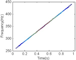
Fig. 3Slice for TFD at t= 0.2 s

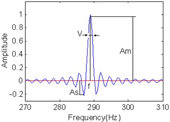
3.2. Construction impact signal model

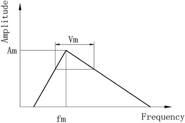
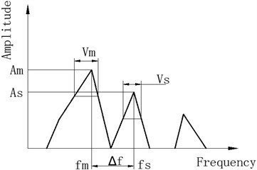
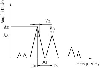
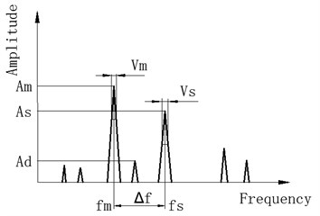
For universal impact signal analysis, the sketch map of frequency-amplitude with frequency cell is shown in Fig. 4 according to the changing process for energy distribution with frequency cells. In the frequency amplitude plane, $A_{m}$ and $A_{s}$ are corresponding to the mainlobe amplitude and sidelobe amplitude, respectively. $V_{m}$ and $V_{s}$ are instantaneous widths corresponding to 0.707 $A_{m}$ and 0.707 $A_{s}$ , respectively. At the same time, $f_{m}$ and $f_{s}$ are instantaneous frequencies corresponding to $A_{m}$ and $A_{s}$ . The distance between $f_{m}$ and $f_{s}$ is within 50 times $V_{m}$ . $A_{m}$ will drop and $A_{s}$ will increase because energy is dispersive with frequency cell growth. $A_{m}$ and $A_{s}$ can be clearly separated when the frequency cell is enough. There will be $A_{d}$ between $A_{m}$ and $A_{s}$ if the frequency cell is further improvement. It is the reason that frequency energy will separate from main lobe and side lobe when frequency cell is very large. It will be corresponding to different instantaneous frequency as frequency cell is very high. It leads to separate to small instantaneous frequency. Otherwise, there is not $A_{d}$ shown as Fig. 4(a)-(c).

If the frequency cell number is small, it is difficult to distinguish different IF characteristics on HS plane. Moreover, energy will disperse with frequency cell number increasing. Some small energy information cannot be shown in the HS. It is not very good for HSA if the frequency cell is very high or very low according to Fig. 4. Therefore, there is the best FR for HSA. Based on above analysis, there is the maximum for $A_{s}$ / $A_{m}$ . At the same time, the scope for $A_{s} / A_{m}$ belongs to [0 1]. To distinguish $A_{s}$ and $A_{m}$ , Eq. (7) must be satisfied:

7

f_{s} - V_{s} / 2 > f_{m} + V_{m} / 2 .

Fig. 4Sketch map of parameters varied with frequency cells increment

a) Low frequency cell

b) Medium frequency cell

c) High frequency cell

d) Very high frequency cell

It can be further expressed as Eq. (8):

8

Δ f = |f_{s} - f_{m}| > (V_{m} + V_{s}) / 2 = V .

$V / Δ f$ is the instantaneous bandwidth. At the same time, it belongs to [0 1]. The smaller is $V / Δ f$ , the better is to distinguish the two peak value $A_{s}$ and $A_{m}$ in the HS plane. Thus, new estimation model must include the two parameters $V / Δ f$ and $A_{s} / A_{m}$ to determine the best FR. At the same time, there will be $A_{d}$ when the FR is very small shown as Fig. 4(d). In this condition, the energy will disperse and the frequency cell number is very high. It is better to reduce $A_{d}$ because it will affect HSA result. It means that the smaller is $A_{d} / A_{m}$ , the better is HSA. Therefore, it is very important to construct an estimation model for TFD to determine the best FR. According to the effect from parameters $V / Δ f$ , $A_{s} / A_{m}$ and $A_{d} / A_{m}$ on FR, new performance estimation models for impact signal are put forward in one amplitude-frequency plane shown in Eq. (9)-(12):

9

p_{1} = (1 - \frac{V}{Δ f}) ∙ \frac{A_{s}}{A_{m}},

10

p_{2} = \frac{((1 - \frac{V}{Δ f}) + \frac{A_{s}}{A_{m}})}{2},

11

p_{3} = \frac{((1 - \frac{V}{Δ f}) + \frac{A_{s}}{A_{m}} + \frac{A_{d}}{A_{m}})}{3},

12

p_{4} = (1 - \frac{V}{Δ f}) \frac{A_{s}}{A_{m}} \frac{A_{d}}{A_{m}} .

Eq. (9) and Eq. (10) don’t consider the small energy separation from the main lobe or side lobe. Eq. (11) and Eq. (12) include $A_{d}$ to performance estimation. Every equation is just suitable for one frequency-amplitude estimation from Eq. (9) to Eq. (12). For the whole time domain, it needs normalized resolution performance measurement. Therefore, Eq. (9)-(12) can be further rewritten as Eq. (13)-(16):

13

p_{11} (t) = \frac{\frac{A_{s j} (t)}{A_{m j} (t)}}{\underset{1 \leq k \leq K}{M a x} (\frac{1}{N} \sum_{t = 1}^{N} \frac{A_{s k} (t)}{A_{m k} (t)})} * (1 - \frac{\frac{V_{j} (t)}{Δ f_{j} (t)}}{\underset{1 \leq k \leq K}{M a x} (\frac{1}{N} \sum_{t = 1}^{N} \frac{V_{k} (t)}{Δ f_{k} (t)})}),

14

p_{22} (t) = \frac{1}{2} (\frac{\frac{A_{s j} (t)}{A_{m j} (t)}}{\underset{1 \leq k \leq K}{M a x} (\frac{1}{N} \sum_{t = 1}^{N} \frac{A_{s k} (t)}{A_{m k} (t)})} + 1 - \frac{\frac{V_{j} (t)}{Δ f_{j} (t)}}{\underset{1 \leq k \leq K}{M a x} (\frac{1}{N} \sum_{t = 1}^{N} \frac{V_{k} (t)}{Δ f_{k} (t)})}),

15

p_{33} (t) = \frac{1}{3} (\frac{\frac{A_{s j} (t)}{A_{m j} (t)}}{\underset{1 \leq k \leq K}{M a x} (\frac{1}{N} \sum_{t = 1}^{N} \frac{A_{s k} (t)}{A_{m k} (t)})} + \frac{\frac{A_{d j} (t)}{A_{m j} (t)}}{\underset{1 \leq k \leq K}{M a x} (\frac{1}{N} \sum_{t = 1}^{N} \frac{A_{d k} (t)}{A_{m k} (t)})}

+ 1 - \frac{\frac{V_{j} (t)}{Δ f_{j} (t)}}{\underset{1 \leq k \leq K}{M a x} (\frac{1}{N} \sum_{t = 1}^{N} \frac{V_{k} (t)}{Δ f_{k} (t)})}),

16

p_{44} (t) = \frac{\frac{A_{s j} (t)}{A_{m j} (t)}}{\underset{1 \leq k \leq K}{M a x} (\frac{1}{N} \sum_{t = 1}^{N} \frac{A_{s k} (t)}{A_{m k} (t)})} * \frac{\frac{A_{d j} (t)}{A_{m j} (t)}}{\underset{1 \leq k \leq K}{M a x} (\frac{1}{N} \sum_{t = 1}^{N} \frac{A_{d k} (t)}{A_{m k} (t)})}

* (1 - \frac{\frac{V_{j} (t)}{Δ f_{j} (t)}}{\underset{1 \leq k \leq K}{M a x} (\frac{1}{N} \sum_{t = 1}^{N} \frac{V_{k} (t)}{Δ f_{k} (t)})}),

where, $t$ is different time slice in the HS plane. $K$ is a set of different frequency number. The normalized resolution performance measure can be used to determine the best FR for HSA.

3.3. Simulation analysis

For a frequency modulation signal, it can be expressed as Eq. (17):

17

x (k) = e x p (- a t) s i n 2 π f_{1} k T,

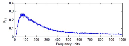
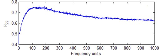
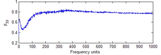
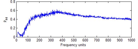
where, $t = m o d (k T, 1 / f_{m}),$ $a =$ 800, $f_{m} =$ 20 Hz, $f_{1} =$ 4000 Hz, $T =$ 1/25600 s, $a$ , $f_{m}$ , $f_{1}$ , $f_{2}$ , $T$ are corresponding to index frequency, modulation frequency, carrier frequency and sampling interval. According to the simulation process, an impact signal can be obtained shown in Fig. 5. Obviously, it belongs to typical nonstationary signal. For more convenient signal analysis and method verification, the second impact process of the simulation signal is intercepted and used for further analysis shown as Fig. 6(a). The total data length is 1024 points for analysis. Ten IMFs can be obtained by using EEMD. Cross-correlation coefficients were calculated for different IMFs corresponding to original signal shown as Table 1. It is obvious that the first IMF has close relationship with original signal and wide frequency band. Thus, it can be used for further analysis to determine the best FR. It can be determined different IMFs according to above equations. But it is difficult to obtain the best FR if all the IMFs are considered. Thus, the first IMF is used to determine the best FR in this research. Different estimation models Eq. (13)-(16) are used to determine the best FR shown in Fig. 7.

Fig. 5Simulation impact signal

Fig. 6Original signal and its corresponding IMFs by using EEMD

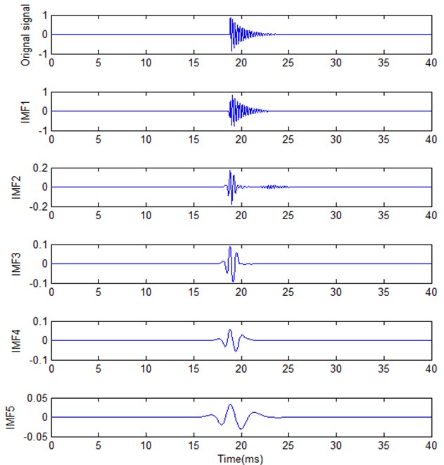
Table 2 provides the result for different best FR based on above estimation models. Fig. 7 provides different calculation result based on new estimation models corresponding to Eq. (13) to Eq. (16). It is obvious that different estimation models are corresponding to different results. According to Fig. 7 and Table 2, $p_{11}$ and $p_{22}$ are not very well compared with $p_{33}$ and $p_{44}$ . It is not convenient for IF analysis because the frequency cells are very low in HS plane. $p_{33}$ and $p_{44}$ have the same result based on Eq. (18) and Eq. (19). But Eq. (19) has good trend with frequency cell number increasing. Thus, it is better for the best FR determination. Compared with other models, $p_{44}$ is more powerful for the best FR determination because it has good performance with FR unit increment according to Fig. 7. It is suitable to determine the best FR in HS analysis as a performance estimation model. At the same time, there is not much difference for frequency cell number from 300 to 400 according to Fig. 7. It is also the reason that there is not much difference for signal analysis from visual inspection. But it has much difference with frequency number from 50 to 100. It is why the FR should not be optionally selected. There will be the best FR for HS analysis.

Table 1Cross-correlation coefficient for every IMF with original signal

	IMF1	IMF2	IMF3	IMF4	IMF5
Cross-corrlation coefficicent	0.9651	0.2509	0.0908	0.1239	0.0763

Table 2Best FR unit number for different estimation model

Estimation model	$p_{11}$	$p_{22}$	$p_{33}$	$p_{44}$
Best FR units number	66	192	352	352

Fig. 7Calculation results based on different estimation model

a) Model with Eq. (13)

b) Model with Eq. (14)

c) Model with Eq. (15)

d) Model with Eq. (16)

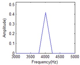
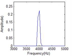
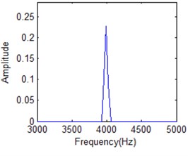
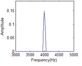
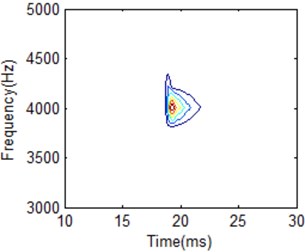
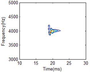
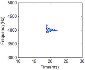
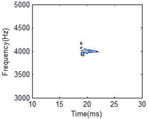
Fig. 8 is a slice of HS when time is 15 milliseconds with different resolution units. It is obvious energy peak value reduces when FR number increases. It means that energy disperses when frequency cell number increases. Fig. 9 is the HS for IMF1 based on different FR. It has the same characteristics for Fig. 8. Moreover, HS is not good to show low energy distribution when the frequency cell is high. Thus, there is a best FR for signal analysis. It is better to select the best FR for signal analysis and feature extraction.

Fig. 8Slice of HS at 15 milliseconds with different resolution units: a) 50, b) 200, c) 352, d) 500

a)

b)

c)

d)

Fig. 9HS for IMF1 with different frequency cells: a) 50, b) 200, c) 352, d) 500

a)

b)

c)

d)

3.4. The best frequency resolution selection algorithm

According to above investigation, it can be concluded that a new estimation model Eq. (16) is suitable to the best FR determination for HS. The process is as following:

1) Using EEMD to obtain IMFs for the original signal.

2) Cross-correlation coefficient calculation for every IMF, determine the IMF for further FR analysis.

3) Calculate different $(1 - V / Δ f)$ , $A_{s} / A_{m}$ , $A_{d} / A_{m}$ for different time slice in a HS.

4) Normalized frequency resolution measure by using Eq. (16).

5) Determine the best FR according to normalized frequency resolution measure.

6) Calculate HS based on the best FR for signal analysis.

According to above analysis, there is not much difference for the frequency cell within a scope according to the simulation signal analysis. The performance measure is very similar for frequency cell number from 300 to 400. It will be difference for the different signal analysis although it is in the same working condition. But the best FR will be within the scope. Therefore, it doesn’t need to calculate FR for every HS during signal analysis in practical application. For one kind of signal analysis, it can just calculate the best FR once by using constructed model. Then, the best FR can be used to analyze this type signal. It can effectively save time and reduce calculation. At the same time, it also improves the classification result based on the best FR analysis. Therefore, it will be more useful for practical signal analysis and machine working condition classification.

4. Application for estimation model

4.1. Experiment and data acquisition

The working condition of combustion system classification for a marine diesel engine is used an experiment to testify the effectiveness of this method. It is an operational marine diesel. In this experiment. diesel engine is as power for the propeller and gearbox is as the power transmission. The schematic diagram is shown as Fig. 10. Experimental picture for diesel engine cylinder head is shown as Fig. 11. Data acquisition system is PDM2000 shown as Fig. 12. It is a two-channel data gathering system which is developed by Institute of Vibration Engineering, Dalian University of Technology. The main parameters of the diesel engine are shown in Table 3.

Fig. 10Schematic diagram for data acquisition

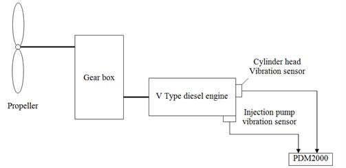
Table 3Main parameters of the marine diesel

Model	PC2-5
Engine type	4-stroke, 12-cylinder, turbocharger
Bore size	400 mm
Stroke	460 mm
Frame	Separated structure
Rated power	5816.46 kW
Rated speed	500 (RPM)

Vibration sensors were located on the cylinder head and injection pump since all cylinder heads are separated, influence from a fault working condition cylinder to its adjacent cylinders is a minimum. Thus, vibration signal measured from a cylinder head can be considered a reprievable signal for the working condition of a cylinder, including combustion and fuel injection, etc. In this research, two types of engine vibration signals were measured under the condition shown in Table 4. One is from a cylinder in normal working condition. The other is from a cylinder where fuel leaking in the injection pipe at the injector end was set as an engine fault. Fuel injection leaking will lead to deteriorate of the combustion process. Its vibration signal from cylinder head will vary from normal working condition. Therefore, the vibration signal from cylinder head could be used for condition classification and fault diagnosis. Table 4 provides the testing condition parameters for this experiment.

Table 4Data sampling parameters

Data length	Crankshaft speed	Analysis frequency	Sampling frequency
32 K	420 RPM	10000 Hz	25600 Hz

Fig. 11Experimental picture

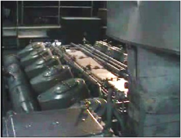
Fig. 12Data acquisition system PDM2000

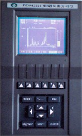
Fig. 13Marine diesel engine cylinder head vibration signal in temporal domain

a) Normal condition

b) Fuel leakage condition

Fig. 13 shows the two time domain vibration signals measured in one engine cycle under the normal and fault conditions. In Fig. 13, CPI stands for combustion process impulse response which contains fuel injection impulse and combustion cylinder pressure impulse, OVC stands for exhaust valve close impulse response, TI stands for throttle force impulse response and IVC stands for inlet valve close response. The complex of the physical and chemical processes during the combustion period, movement of valves and pistons make the signals fluctuate during a cycle and the difference in the max amplitude, which is also affected by noise contained in the signals. It is very difficult to distinguish the two working conditions just according to the temporal domain analysis. There is not any clear information between normal working condition and fuel leakage condition. Thus, further research should be carried on for machine working condition pattern recognition.

Mathematically, the relationship between a vibration signal $Y (t)$ of a linear time-invariant system and its signal vibration source $X (t)$ can be simplified and expressed by Eq. (18). For the diesel engine cylinder head vibration signal, it can be shown in Fig. 14:

18

Y (t) = h (t) * X (t),

where, $h (t)$ is the impulse response path of $X (t)$ .

Fig. 14Model of cylinder head vibration

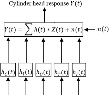
In Fig. 14, $h_{J} (t)$ , $h_{C} (t)$ , $h_{O} (t)$ , $h_{T} (t)$ stand for the response paths of injection pressure, combustion pressure, exhaust valve close, throttle impulse and inlet valve close. At the same time, the vibration signals generated by impulse forces follow a fixed time regularity in every engine working cycle. Thus, the impulse response actions in the time domain can be separated according to their individual characteristics [12-14]. According to the diesel engine working principles, the event of the vibration responses during the combustion period is shown as Fig. 14. It could be divided into three stages. Stage 1: no impulse response; Stage 2: fuel injection impulse response; and Stage 3: combustion process impulse response. For the combustion process, it contains lots of information about the diesel engine working conditions. It can be further used for diesel engine working condition classification and fault diagnosis. As for the fuel injection fault condition, the injection process will have effect the combustion process, so does its vibration signal. The combustion stage could be used for condition classification in this research.

4.2. Best frequency resolution determination

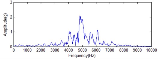
The total length obtained from the combustion process for further investigation is 1024 points. By using EEMD process, diesel engine vibration signal during the combustion process for normal and fuel leakage working condition can be shown in Fig. 15 and Fig. 16, respectively. Table 5 provides the related cross-correlation coefficients with original signal. It is very obvious that IMF1 is very similar to original signal for every working condition. It contains a lot of information. EMD can be looked on as a filter [15], so does the EEMD. Its frequency band scope will be different for the IMFs. The first IMF has identical frequency band with original signal according to Fig. 15 and Fig. 16. Fig. 17 shows fast Fourier transform analysis for normal condition signal and its corresponding IMF1. It is obvious that the first IMF has identical frequency band with original signal. At the same time, fuel leakage condition has the same result. As for other IMFs, its frequency band will be shortened. IF doesn’t need high frequency cell number for other IMFs compared with IMF1. Therefore, the first IMF can be used to determine the best FR for HSA. Moreover, the whole signal HS is calculated from the Hilbert transform for every IMF. It must be demonstrated by every IMF clearly which can give more information about signal characteristics. Thus, IMF1 for the normal and fuel leakage condition can be used to determine the best frequency cells.

Fig. 15Normal signal and its corresponding IMFs by using EEMD process

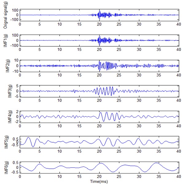
Table 5Cross-correlation coefficient for every IMF with original signal for different conditions

Cross-correlation coefficient	IMF1	IMF2	IMF3	IMF4	IMF5	IMF6
Normal condition	0.9807	0.2168	0.1006	0.0394	0.0235	0.0189
Fuel leakage	0.9731	0.2122	0.0397	0.0242	0.0183	0.0272

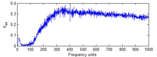
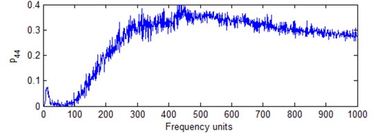
IMF1 of the two conditions were used to determine the best FR. Fig. 18 shows normalized FR estimation measure with frequency cell number for the two different conditions according to Eq. (19). For the normal condition, the best frequency cell is 404. For the fault condition, the best frequency cell is 440. Although there is a little difference for the best frequency cell, the difference for FR measure is very small according to the normalized measure shown in Fig. 18. In practical signal analysis, it is not impossible to have the same best frequency cell for two different signals. As stated above, a best frequency cell can be selected and applied to other related signal analysis.

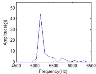
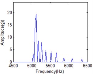
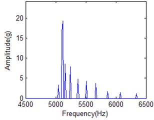
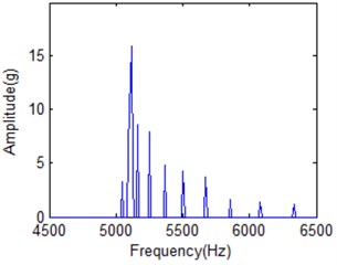
Fig. 19 shows amplitude-frequency spectrum of IMF1 under different frequency cell when time is 20 ms for normal condition IMF1. It is obvious that energy distribution disperses with frequency cell increasing. When frequency number is 50, energy is concentrated. It is difficult to distinguish different IF. It will be better for frequency cell is 200. But it is obvious that there is IF cannot separated from the main lobe shown in Fig. 19(b). All the IFs can be classified in Fig. 19(c) when it is in the best FR condition. When frequency cell is 500, all the IFs can also be distinguished. But its energy will be further dispersive as shown in Fig. 19(d). It will affect the classification result. It also means there is the best FR for HS based on above analysis.

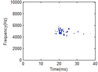
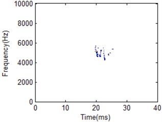
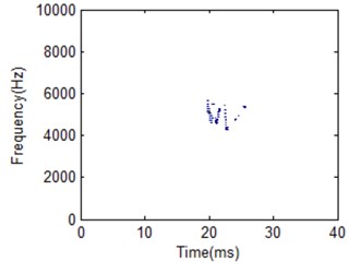
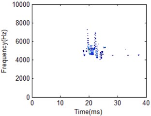
Fig. 20 shows HSA based on IMF1 for normal condition with different frequency cells. The energy shown in Fig. 20(a) is concentrated because the frequency cell is very low. It is difficult to separate different IF. It is also the reason that the combustion process is longer compared with Fig. 20(b). It can be looked as delay combustion. Thus, it is not very good for practical signal analysis. At the same time, Fig. 20(d) is dispersed as frequency cell number is high. At the same time, the frequency band is also wider. In practical signal analysis, there is the best frequency cell number. The more or the less cannot provide accurate result. Moreover, it will affect analysis process. Fig. 20(b) and Fig. 20(c) is very identical although frequency cell is 404 or 440, respectively. That also means there is not much difference for HS within a frequency cell scope. FR must be selected during the HS analysis. The best FR will be convenient for practical signal analysis.

Fig. 16Fuel leakage condition signal and its corresponding IMFS by using EEMD process

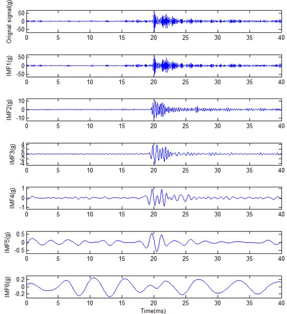
Fig. 17Fast Fourier transform analysis for original signal and its corresponding IMF1

a) Original signal

b) IMF1

Fig. 18HS of the overall signal under different frequency cell

a) Normal working condition

b) Fuel leakage condition

Fig. 19The amplitude-frequency spectrum of IMF1 under different frequency cell when time is 20 milliseconds

a) 50 frequency cells

b) 200 frequency cells

c) 404 frequency cells

d) 500 frequency cells

4.3. Hilbert spectrum classification by using the best frequency resolution

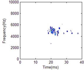
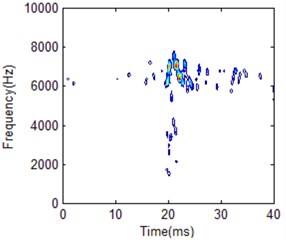
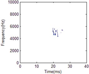
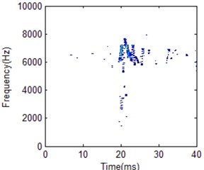
The vibration frequency due to diesel engine combustion varies with the structure of the engine. Particularly, the combustion chamber structure and the materials of the engine components affect transmission speed of vibration. The cylinder head vibration frequency band for diesel engine combustion is mainly concentrated on the middle and low band [16]. When the diesel engine operates in failure condition, its energy distribution in terms of time and frequency information will vary from the normal condition. This is an important feature for diesel engine pattern recognition and fault diagnosis. It can be used for diesel engine working condition classification and fault diagnosis. 404 frequency cellis used to construct the whole HS for the two different working conditions classification. Fig. 21 to Fig. 23 gives the comparison for the two working conditions with different frequency cell.

Fig. 20HS of IMF1 under different frequency cell number for normal condition

a) 50 frequency cells

b) 404 frequency cells

c) 440 frequency cells

d) 500 frequency cells

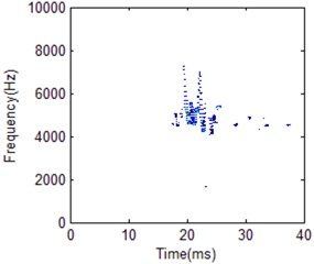
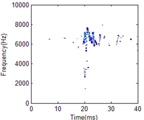
It is obviously the two different working conditions corresponding to different HS. But the classification result by using different FR is also different. Frequency cell 404 is better for two working condition recognition according to the comparison shown in Fig. 22. Its frequency band is between 4000 to 6000 Hz for normal condition. For low frequency cell 50 shown in Fig. 21, energy distribution is very concentrated which makes the main impact information wider in time domain compared with the best FR HS. On the other hand, energy distribution is more dispersive for frequency cell 500 shown in Fig. 23. It makes the main impact information in frequency domain wider compared with the best FR HS. Its frequency band is between 4000 to 8000 Hz. It is a little similar with fuel leakage condition. Thus, it will influence classification result. For the fuel leakage condition, it will lead to the combustion deterioration, so does the impact vibration reduction. At the same time, its HS distribution is dispersive.

From the analysis results, the vibration frequency caused by combustion process of the test engine is within medium and low band. HS for fuel leakage condition is with high frequency band. It will be helpful to determine information whether machine is working in normal condition or not. It is proved that this is caused by injection delay and poor fuel atomisation which, in most case, is a result of fuel injection system leaking. Thus, the best FR can be helpful for fault condition classification compared with other FR.

HS is beneficial to demonstrate signal nonstationary features. But its frequency resolution is important parameters for feature extraction and fault diagnosis. As for now, the limitation introduction for FR is only demonstrated by Huang [3]. It is urgently needed further improvement. According to the parameters analysis for FR estimation in this paper, $(1 - V / Δ f)$ , $A_{s} / A_{m}$ , $A_{d} / A_{m}$ in an amplitude-frequency plane are considered to construct performance model for FR determination. All these parameters are closed related with FR. These parameters can be used to estimate the performance of FR. Thus, the estimation model can demonstrate the relationship different parameters. It is beneficial to determine the best suitable estimation model. Compared with frequency determination based on visual, the estimation model put forward in this research can more accurate to select the best FR for pattern recognition. This can be helpful to determine the suitable FR to construct HS which has great influence on recognition result.

Fig. 21HS comparison for different working conditions with 50 frequency cells

a) Normal condition

b) Fuel leakage condition

Fig. 22HS comparison for different working conditions with 404 frequency cells

a) Normal condition

b) Fuel leakage condition

Fig. 23HS comparison for different working conditions with 500 frequency cells

a) Normal condition

b) Fuel leakage condition

5. Conclusions

In this paper, a new method to estimate the performance of HS based on the best FR determination is demonstrated in detail. Simulated signal and practical testing diesel engine vibration signal are used to testify the effectiveness of this model. The results confirmed that this model is helpful to determine the best FR for HS. The improved HS based on estimation model is also beneficial to feature extraction and fault diagnosis. At the same time, this estimation model needs more verification and application for practical signal analysis. Further research will be carried on the performance estimation model improvement for FR. Different parameters will be considered during model construction process. As well, practical application investigation will also be carried on for HS based on performance estimation model analysis.

References

He Z., Zi Y., Chen X. Some scientific issues in mechanical fault diagnosis. Journal of Vibration and Shock, Vol. 31, Issue 6, 2009, p. 144-147.

Search CrossRef
Peng Z. K., Chu F. L., Tse P. W.. Detection of the rubbing-caused impacts for rotor-stator fault diagnosis using reassigned scalogram. Mechanical Systems and Signal Processing, Vol. 19, Issue 2, 2005, p. 391-409.

Search CrossRef
Huang N. E., Shen Z., Long S. R. The empirical mode decomposition and the Hilbert spectrum for nonlinear and non-stationary time series analysis. Proceedings of The Royal Society of London Series A- Mathematical Physical And Engineering Sciences, Vol. 454, Issue A, 1998, p. 903-995.

Search CrossRef
Li H., Zhou P., Zhang Z. An investigation into machine pattern recognition based on time-frequency image feature extraction using a support vector machine. Journal of Mechanical Engineering Science, Vol. 224, Issue 4, 2040, p. 981-994.

Search CrossRef
Wu Z., Schneider E. K., Kirtman B. P., Sarachik E. S., Huang N. E., Tucker C. J. The modulated annual cycle: an alternative reference frame for climate anomalies. Climate Dynamics, Vol. 31, Issue 7-8, 2008, p. 823-841.

Search CrossRef
Zhang R. R., Ma S., Safak E., Hartzell S. Hilbert-Huang transform analysis of dynamic and earthquake motion recordings. Journal of Engineering Mechanics, Vol. 129, Issue 8, 2003, p. 861-875.

Search CrossRef
Wu Z., Huang N. E. Ensemble empirical mode decomposition: A noise-assisted data analysis method. Advances in Adaptive Data Analysis, Vol. 1, Issue 1, 2009, p. 1-41.

Search CrossRef
Li H., Zhang Z. Frequency resolution effect on hilbert spectrum for instantaneous vibration impact signal analysis. Key Engineering Materials, Vol. 413-414, 2009, p. 135-142.

Search CrossRef
Boashash B. Time frequency signal analysis and processing: a comprehensive reference. Oxford, UK, Elsevier, 2003.

Search CrossRef
Barkat B., Boashash B. A high-resolution quadratic time–frequency distribution for multicomponent signals analysis. IEEE Transactions on Signal Processing, Vol. 49, Issue 10, 2001, p. 2232-2239.

Search CrossRef
Boashash B., Sucic V. Resolution measure criteria for the objective assessment of the performance of quadratic time-frequency distributions. IEEE Transactions on Signal Processing, Vol. 51, 2003, p. 1253-1263.

Search CrossRef
Antoni J., Daniere J., Guillet F. Effective vibration analysis of IC engines using cyclostationarity. Part I – A methodology for condition moitoring. Journal of Sound and Vibration, Vol. 257, Issue 5, 2002, p. 815-837.

Search CrossRef
Antonia J., Danierea J., Guilleta F., Randallb R. B. Effective vibration analysis of IC engines using cyclostationarity. Part II – New results on the reconstruction of the cylinder pressures. Journal of Sound and Vibration, Vol. 257, Issue 5, 2002, p. 839-856.

Search CrossRef
Johnsson R. Cylinder pressure reconstruction based on complex radial basis function networks from vibration and speed signals. Mechanical Systems and Signal Processing, Vol. 20, Issue 8, 2006, p. 1923-1940.

Search CrossRef
Wu Z., Huang N. E. A study of the characteristics of white noise using the empirical mode decomposition method. Proceedings of The Royal Society of London Series A- Mathematical Physical and Engineering Sciences, Vol. 460, 2004, p. 1597-1611.

Search CrossRef
Li H., Zhou P., Ma X. Marine diesel engine fault diagnosis by using improved Hilbert spectrum. Journal of Ship Research, Vol. 50, Issue 4, 2006, p. 378-387.

Search CrossRef

About this article

Received

18 June 2014

Accepted

07 September 2014

Published

30 September 2014

Keywords

Hilbert spectrum

frequency resolution

estimation model

instantaneous impact signal

Acknowledgements

The support from Chinese National Science Foundation (Grant No. 50805014 and No. 51175057) and the Fundamental Research Funds for the Central Universities (Grant No. DUT14ZD204) for this research is gratefully acknowledged. The anonymous reviewers are sincerely appreciated for their valuable comments and suggestions to improve the paper.

This is an open access article distributed under the Creative Commons Attribution License, which permits unrestricted use, distribution, and reproduction in any medium, provided the original work is properly cited.