Receptance coupling for frequency response prediction of cylindrical workpiece in CNC lathe

Li, Hui; Xue, Gang; Zhou, Yang; Li, He; Wen, Bangchun

Journal of Vibroengineering

Browse Journal

Submit article

Published: 30 June 2015

Check for updates

Receptance coupling for frequency response prediction of cylindrical workpiece in CNC lathe

Hui Li¹

Gang Xue²

Yang Zhou³

He Li⁴

Bangchun Wen⁵

^{1, 4, 5}School of Mechanical Engineering & Automation, Northeastern University, Shenyang, 110819, China

²Siemens Electrical Drives Ltd., Tianjin, 300192, China

³Weichai Power Co., Ltd., Zhejiang, 310030, China

Corresponding Author:

Hui Li

Cite the article Download PDF

Downloads 1693

WoS Core Citations 3

Abstract

Receptance coupling method was often used to predict frequency response function (FRF) at the tool point of CNC milling. In this paper, it was applied in the frequency response prediction of cylindrical workpiece in CNC lathe. In order to improve prediction accuracy, receptance pre-experiment method was proposed to obtain 2×2 receptance matrix of chuck section which represented the most crucial coupling receptance of the workpiece-chuck assembly. In this method, FRF measurement of a “calibration shaft” inserted in the chuck was combined with some numerical calculations to obtain translational and rotational receptance data which reflected coupling dynamics between the workpiece and the chuck. Besides, some major influences on the receptance matrix of chuck section were experimentally analyzed, such as impact distance, free length, clamping length, diameter of calibration shaft and its real clamping effect, so that we can find out an appropriate calibration shaft to ensure the accuracy of receptance matrix of chuck section. At last, practicability and efficiency of receptance coupling method had been demonstrated by a verification case using a stepped cylindrical workpiece as the object machined in CAK3675 lathe. The predicted direct and cross FRF were observed to have a good agreement with measured results.

1. Introduction

Cylindrical workpiece is often machined into different sizes of shaft by CNC lathe, such as axle shaft, stepped shaft, taper shaft and hollow shaft. The frequency response function (FRF) of these machined shafts or cylindrical workpiece can indicate dynamic characteristics of the workpiece-chuck assembly and it is frequently applied in the area of structural modification and finite element model updating [1]. Besides, it is a crucial parameter for the stability lobe diagram which identifies stable and unstable cutting zones as a function of the chip width and spindle speed [2]. Therefore, successfully obtaining accurate FRFs data will be of much help to fault diagnosis, dynamic response analysis, cutting optimization, performance evaluation and etc. Impact modal testing can directly measure the workpiece’s FRFs, but the pulse signal and response signal measured by accelerometer or no-contact sensor are inevitably affected and interfered by background noise in the process of measurement and signal transmission, especially when the noise pollution is serious (often occurred in machining plant and assembly plant where CNC lathe is operated), the accuracy of FRFs data will be greatly reduced [3]. Another problem is that FRF measurement is a time-consuming process, including attaching transducers to the measuring points, recording and saving measured signals, adopting some data processing techniques (e.g. filtering, windowing, smoothing, spectral analysis) to get the final test results and etc. Meanwhile, it is unfeasible to carry out FRF measurement every time if different sizes of workpiece (with different diameter or length) are frequently installed in the CNC lathe. Therefore, further research efforts on predicting FRFs of cylindrical workpiece are still needed, particularly, providing some analytical or simulation methods with high practicability and efficiency.

Bishop [4] firstly proposed receptance coupling method in his book. Schmitz et al. [5-6] have further developed this theory and applied it on the field of high-speed machining dynamics prediction as well as the field of chatter recognition and control. For instance, they treated the tool-holder-spindle assembly as separate substructures, i.e. the tool and the holder-spindle, and employed receptance coupling substructure analysis (RCSA) to predict the tool point dynamic response by combining frequency response measurements of individual components through appropriate connections. Later Schmitz et al. [7-9] employed the concept of multi-point coupling to provide more accurate models of the joint interfaces stiffness and damping. Schmitz et al. [10] also proposed a new experimental method to determine the character of the real portion of FRF in the tool point of high-speed machining by sampling the tool displacement at peak force, where an optical displacement sensor was used as the response sensor and non-contact magnetic the force sensor was placed in close proximity to the tool point.

Park et al. [11] presented an improved receptance coupling technique to identify the end mill-spindle/tool holder joint dynamics, which included both translational and rotational degrees of freedom. Three blank cylinders with different length were mounted with a set length to the tool holder, the short cylinder was used to identify the spindle–tool holder assembly dynamics, and the long cylinder was used to identify the joint parameters. Finally, the rotational dynamics of the end mill-spindle assembly were extracted mathematically from the direct and cross FRF measurements applied to the medium cylinder. But the author did not discuss the influences of the length of blank cylinder on the accuracy of receptance coupling. Besides, they did not give quantified formula to help choose appropriate cylinder. Erturka et al. [12] used receptance coupling and structural modification techniques to calculate the tool point FRF in a machining center so that chatter stability analysis can be done. They believed that spindle, holder and tool were not slender enough to neglect the effects of shear deformation and rotary inertia, so Timoshenko beam theory was used for modeling their dynamics, and contact stiffness and damping representing the joint between these components had been considered as well. Ahmadi and Ahmadian [13] took into account the change in normal stiffness along the tool shank part and proposed a new approach in modeling high-speed machining dynamics by using the measured dynamic flexibility of the holder–spindle assembly and an analytic model for the tool. Modal tests in the tool tip were performed by an impact hammer and the measured FRFs were employed in identifying the joint interface parameters. Zhang et al. [14] divided the machine-spindle-holder-tool assembly into three parts, including holder and tool shank, machine-spindle and the fluted portion. Consequently, dynamic responses in the tool point were predicted using the receptance coupling technique. The receptances for the fluted portion of the tool were calculated by FEM and an equivalent beam diameter Timoshenko model. The tool shank and holder receptances were also modeled using Timoshenko beam theory, while the machines-spindle receptances were measured by impact testing. Catania and Mancinelli [15] proposed a model of the milling machine-tool, the machine frame and the spindle were modeled by an experimentally evaluated modal model, several FRFs were collected by exciting the tool and the spindle of 4 axis NC milling machine with an instrumented impact hammer. FRFs results were used as important inputs to calculate the stability lobe charts. Besides, natural frequencies and modal damping ratios were identified from the resulting FRFs by a least square complex method.

However, the above studies made by scholars and researchers were mainly focused on the FRF prediction of tool point of CNC milling or machining center, prediction studies on FRFs of cylindrical workpiece in CNC lathe were still rare. This research described the application of receptance coupling method to the analytic prediction of FRFs of cylindrical workpiece with different diameters and lengths. In order to overcome the limitations in traditional calculation methods and improve the prediction accuracy, receptance pre-experiment method was proposed to obtain 2×2 receptance matrix of chuck section which represented the most crucial coupling receptance of the workpiece-chuck assembly. In this method, FRF measurement of a “calibration shaft” inserted in the chuck was combined with some numerical calculations to obtain translational and rotational receptance data which reflected coupling dynamics between the workpiece and the chuck. Besides, some major influences on the receptance matrix of chuck section were experimentally analyzed, such as impact distance, free length, clamping length, diameter of calibration shaft and its real clamping effect, so that we can find out an appropriate calibration shaft to ensure the accuracy of receptance matrix of chuck section. At last, practicability and efficiency of receptance coupling method had been demonstrated by a verification case using a stepped cylindrical workpiece as the object machined in CAK3675 lathe. The predicted direct and cross FRF were observed to have a good agreement with measured results, and the predicted FRF has a broad application prospect in the field of dynamic response analysis, finite element model updating, vibration performance evaluation, cutting chatter prediction and etc.

2. Prediction principle

For a cylindrical workpiece installed in the lathe chuck, its receptance coupling model can be depicted by two individual substructures: substructure $A$ and substructure $B$ , as shown in Fig. 1. Where substructure $A$ represents the free part of the workpiece with length $l^{A}$ and diameter $d^{A}$ , substructure $B$ is consist of the clamped part of the workpiece (clamping length is $l^{B}$ ) and lathe chuck. And number 1-3 refer to different cross section of the receptance coupling model, specifically, the free section of the workpiece is represented by 1, the clamped section of the workpiece 2 and the chuck section 3. It should be noted that the reason why the clamped part of the workpiece is divided into substructure $B$ rather than $A$ is that we can get the information on the joint interface between the workpiece and the chuck by receptance pre-experiment method (we will describe it in section 3), which could avoid imprecise or uncertain results of the concerned receptance matrix of chuck section, introduced by some traditional calculation methods.

Fig. 1Receptance coupling model of cylindrical workpiece-chuck assembly

2.1. Substructure receptance

The following will give the principle formulas of substructure receptance by taking substructure $A$ as an example, suppose this substructure can be modeled as an Euler-Bernoulli beam [4], and $X_{1}^{A}$ , $X_{2}^{A}$ , $F_{1}^{A}$ , $F_{2}^{A}$ , $Θ_{1}^{A}$ , $Θ_{2}^{A}$ , $M_{1}^{A}$ , $M_{2}^{A}$ are the displacements, forces, rotations and moments at cross section 1 and 2 respectively, where the directions of the forces and moments are in the same directions of displacements and rotations, as seen in Fig. 2.

Fig. 2The position and direction of the displacement and rotation of beam model

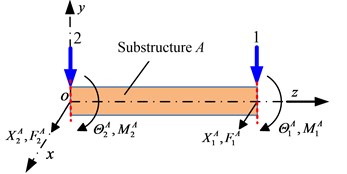
According to receptance coupling principle [4-7], the receptance matrix $R_{j k}^{i} (ω)$ , can be expressed as:

1

R_{j k}^{i} (ω) = [\begin{array}{l} \frac{X_{j}^{i}}{F_{k}^{i}} & \frac{X_{j}^{i}}{M_{k}^{i}} \\ \frac{Θ_{k}^{i}}{F_{k}^{i}} & \frac{Θ_{k}^{i}}{M_{k}^{i}} \end{array}] = [\begin{array}{l} H_{j k}^{i} & L_{j k}^{i} \\ N_{j k}^{i} & P_{j k}^{i} \end{array}],

where, $R_{j k}^{i} (ω)$ is consist of four elements, such as $H_{j k}^{i}$ (displacement/force), $L_{j k}^{i}$ (displacement/moment), $N_{j k}^{i}$ (rotation/force) and $P_{j k}^{i}$ (rotation/moment). The superscript $i$ denotes the different substructure or assembly, because substructure $A$ is the major concern in this example, it can be defined as $i = A$ ; and the subscript $j$ , $k$ denote different cross section of the substructure respectively. For substructure $A$ and its free section 1 and constraint section 2, it can be defined as $j = 1$ , $k = 2$ . If cross section $k$ is coincident with cross section $j$ , the receptance $R_{j k}^{i} (ω)$ is regarded as a direct receptance; otherwise, it is a cross receptance.

Assume that $m^{A}$ is the mass (kg) of substructure $A$ , $ω$ is the frequency (rad/s), $E^{A}$ is the elastic modulus (N/m²), $J^{A}$ is the second area moment of inertia (m⁴), $η$ is the structural damping factor (unitless). Based on motion equation of the beam and its boundary conditions, e.g., the free-free beam in Fig. 2, the direct and cross receptance matrix of substructure $A$ at cross section 1 and 2 can be expressed as:

2

R_{11}^{A} = [\begin{array}{l} H_{11}^{A} & L_{11}^{A} \\ N_{11}^{A} & P_{11}^{A} \end{array}] = [\begin{array}{l} \frac{- W_{5}^{A}}{E^{A} J^{A} W_{3}^{A} λ^{3}} & \frac{W_{1}^{A}}{E^{A} J^{A} W_{3}^{A} λ^{2}} \\ \frac{W_{1}^{A}}{E^{A} J^{A} W_{3}^{A} λ^{2}} & \frac{W_{6}^{A}}{E^{A} J^{A} W_{3}^{A} λ} \end{array}],

3

R_{12}^{A} = [\begin{array}{l} H_{12}^{A} & L_{12}^{A} \\ N_{12}^{A} & P_{12}^{A} \end{array}] = [\begin{array}{l} \frac{W_{8}^{A}}{E^{A} J^{A} W_{3}^{A} λ^{3}} & \frac{- W_{10}^{A}}{E^{A} J^{A} W_{3}^{A} λ^{2}} \\ \frac{W_{10}^{A}}{E^{A} J^{A} W_{3}^{A} λ^{2}} & \frac{W_{7}^{A}}{E^{A} J^{A} W_{3}^{A} λ} \end{array}],

4

R_{21}^{A} = [\begin{array}{l} H_{21}^{A} & L_{21}^{A} \\ N_{21}^{A} & P_{21}^{A} \end{array}] = [\begin{array}{l} \frac{W_{8}^{A}}{E^{A} J^{A} W_{3}^{A} λ^{3}} & \frac{W_{10}^{A}}{E^{A} J^{A} W_{3}^{A} λ^{2}} \\ \frac{- W_{10}^{A}}{E^{A} J^{A} W_{3}^{A} λ^{2}} & \frac{W_{7}^{A}}{E^{A} J^{A} W_{3}^{A} λ} \end{array}],

5

R_{22}^{A} = [\begin{array}{l} H_{22}^{A} & L_{22}^{A} \\ N_{22}^{A} & P_{22}^{A} \end{array}] = [\begin{array}{l} \frac{- W_{5}^{A}}{E^{A} J^{A} W_{3}^{A} λ^{3}} & \frac{- W_{1}^{A}}{E^{A} J^{A} W_{3}^{A} λ^{2}} \\ \frac{- W_{1}^{A}}{E^{A} J^{A} W_{3}^{A} λ^{2}} & \frac{W_{6}^{A}}{E^{A} J^{A} W_{3}^{A} λ} \end{array}],

where:

λ = \sqrt[4]{m^{A} ω^{2} / E^{A} J^{A} l^{A} (1 + i η)}, W_{1}^{A} = s i n (λ l^{A}) s i n h (λ l^{A}),

W_{3}^{A} = c o s (λ l^{A}) c o s h (λ l^{A}) - 1, W_{5}^{A} = c o s (λ l^{A}) s i n h (λ l^{A}) - s i n (λ l^{A}) c o s h (λ l^{A}),

W_{6}^{A} = c o s (λ l^{A}) s i n h (λ l^{A}) + s i n (λ l^{A}) c o s h (λ l^{A}), W_{7}^{A} = s i n (λ l^{A}) + s i n h (λ l^{A}),

W_{8}^{A} = s i n (λ l^{A}) - s i n h (λ l^{A}), W_{10}^{A} = c o s (λ l^{A}) - c o s h (λ l^{A}) .

2.2. Substructure receptance coupling

The following will deduce the principle formulas of substructure receptance coupling, and frequency response prediction principle of cylindrical workpiece can be clarified during the derivation process.

2.2.1. Direct FRF prediction

Usually, when the FRFs is tested or predicted by experimental or analytical method, it is essential to determine one or more excitation point positions as well as response point positions. For the direct FRF prediction by receptance coupling method, suppose that the concerned excitation point and response point are at the same cross section 4, which divides substructure $A$ into two separated substructures, namely substructure $C$ and substructure $D$ with the related cross section 4 $a$ and 4 $b$ . Receptance coupling model of substructure $B$ and $C$ can be seen in Fig. 3.

Fig. 3Schematic of receptance coupling model between substructure B and substructure C

Suppose that a virtual internal force, $F_{3}^{B}$ is applied on the substructure $B$ at cross section 3, and the corresponding internal displacement can be expressed $X_{3}^{B}$ ; Similarly, $F_{2}^{C}$ is applied on the substructure $C$ at cross section 2, and $X_{2}^{C}$ is the internal displacement. Then, assembly $B C$ (or called the coupled substructure $B C$ ) can be obtained by coupling $B$ and $C$ , suppose that a virtual external force, $F_{3}^{B C}$ is applied on assembly $B C$ at cross section 3 (or cross section 2, if that $F_{2}^{B C}$ would be used), and the corresponding external displacement can be expressed $X_{3}^{B C}$ ; similarly, $F_{4 a}^{B C}$ is applied on assembly $B C$ at cross section 4 $a$ , and $X_{4 a}^{B C}$ is the external displacement.

Considering the relation of force and displacement at cross section 4 $a$ , 2 and 3:

6

[\begin{array}{l} X_{4 a}^{B C} \\ X_{2}^{C} \end{array}] = [\begin{matrix} H_{4 a 4 a}^{C} & H_{4 a 2}^{C} \\ H_{24 a}^{C} & H_{22}^{C} \end{matrix}] [\begin{matrix} F_{4 a}^{B C} \\ F_{2}^{C} \end{matrix}],

7

X_{3}^{B} = H_{33}^{B} F_{3}^{B} .

The equilibrium and compatibility conditions at cross section 4 $a$ , 2 and 3 provide the following boundary conditions:

8a

F_{3}^{B C} = F_{3}^{B} + F_{2}^{C},

8b

X_{3}^{B C} = X_{3}^{B} = X_{2}^{C},

which are used in coupling the substructure $B$ with substructure $C$ .

By considering the compatibility and equilibrium conditions (bring Eq. (8) into Eq. (6) and Eq. (7)), we obtain the following equation:

9a

X_{3}^{B C} = X_{2}^{C} = H_{24 a}^{C} F_{4 a}^{B C} + H_{22}^{C} F_{2}^{C},

9b

F_{3}^{B} = F_{3}^{B C} - F_{2}^{C} = (H_{22}^{C} + H_{33}^{B})^{- 1} (H_{24 a}^{C} F_{4 a}^{B C} + H_{22}^{C} F_{3}^{B C}) .

After simplifying Eq. (9), the displacements $X_{4 a}^{B C}$ and $X_{3}^{B C}$ can be expressed as functions of displacement-to-force receptance $H_{j k}^{i}$ ( $i = C$ , $j$ , $k =$ 4 $a$ or 2) and applied forces $F_{4 a}^{B C}$ and $F_{3}^{B C}$ as follow:

10a

X_{4 a}^{B C} = H_{4 a 4 a}^{C} F_{4 a}^{B C} + H_{4 a 2}^{C} (F_{3}^{B C} - F_{3}^{B}) = H_{4 a 4 a}^{C} F_{4 a}^{B C} + H_{4 a 2}^{C} F_{3}^{B C} - H_{4 a 2}^{C} F_{3}^{B},

10b

X_{3}^{B C} = H_{24 a}^{C} F_{4 a}^{B C} + H_{22}^{C} (F_{3}^{B C} - F_{3}^{B}) = H_{24 a}^{C} F_{4 a}^{B C} + H_{22}^{C} F_{3}^{B C} - H_{22}^{C} F_{3}^{B} .

The equations can be rearranged in a matrix form as follow:

11

[\begin{array}{l} X_{4 a}^{B C} \\ X_{3}^{B C} \end{array}] = [\begin{matrix} H_{4 a 4 a}^{C} - H_{4 a 2}^{C} (H_{22}^{C} + H_{33}^{B})^{- 1} H_{24 a}^{C} & H_{4 a 2}^{C} - H_{4 a 2}^{C} (H_{22}^{C} + H_{33}^{B})^{- 1} H_{22}^{C} \\ H_{24 a}^{C} - H_{22}^{C} (H_{22}^{C} + H_{33}^{B})^{- 1} H_{24 a}^{C} & H_{22}^{C} - H_{22}^{C} (H_{22}^{C} + H_{33}^{B})^{- 1} H_{22}^{C} \end{matrix}] [\begin{array}{l} F_{4 a}^{B C} \\ F_{3}^{B C} \end{array}] .

Extract the first element of the matrix in Eq. (11), we can get $H_{4 a 4 a}^{B C}$ as follow:

12

H_{4 a 4 a}^{B C} = \frac{X_{4 a}^{B C}}{F_{4 a}^{B C}} = H_{4 a 4 a}^{C} - H_{4 a 2}^{C} (H_{22}^{C} + H_{33}^{B})^{- 1} H_{24 a}^{C} .

Similarly, based on the derivation process of Eq. (6) to Eq. (12), we can also get $L_{4 a 4 a}^{B C}$ (displacement/moment), $N_{4 a 4 a}^{B C}$ (rotation/force) and $P_{4 a 4 a}^{B C}$ (rotation/moment), and through combining these receptances with $H_{4 a 4 a}^{B C}$ , we can obtain the 2×2 receptance matrix of assembly $B C$ at cross section 4 $a$ , $R_{4 a 4 a}^{B C}$ as follow:

13

R_{4 a 4 a}^{B C} = [\begin{array}{l} H_{4 a 4 a}^{B C} & L_{4 a 4 a}^{B C} \\ N_{4 a 4 a}^{B C} & P_{4 a 4 a}^{B C} \end{array}] = R_{4 a 4 a}^{C} - R_{4 a 2}^{C} {(R_{22}^{C} + R_{33}^{B})}^{- 1} R_{24 a}^{C},

where, $R_{4 a 4 a}^{C}$ , $R_{4 a 2}^{C}$ , $R_{22}^{C}$ and $R_{24 a}^{C}$ can be calculated by reference to the derivation process of Eq. (1) to Eq. (5), and the receptance matrix of chuck section, $R_{33}^{B}$ , can be obtained by receptance pre-experiment method, we will introduce this method in section 3.

Fig. 4Schematic of receptance coupling model between assembly BC and substructure D

After $R_{4 a 4 a}^{B C}$ is deduced, again, couple assembly $B C$ with substructure $D$ and their receptance coupling model can be seen in Fig. 4, and suppose that a virtual external force, $F_{4}^{B C D}$ is applied on the assembly $B C D$ at cross section 4 and the corresponding external displacement can be expressed $X_{4}^{B C D}$ ; similarly, suppose that a virtual internal force, $F_{4 b}^{D}$ is applied on the substructure $D$ at cross section 4 $b$ , and the corresponding internal displacement can be expressed $X_{4 b}^{D}$ .

Considering the relation of force and displacement at cross section 4 $a$ , 4 $b$ and 4:

14

H_{4 a 4 a}^{B C} = \frac{X_{4 a}^{B C}}{F_{4 a}^{B C}},

15

H_{4 b 4 b}^{D} = \frac{X_{4 b}^{D}}{F_{4 b}^{D}},

16

H_{44}^{B C D} = \frac{X_{4}^{B C D}}{F_{4}^{B C D}} .

The equilibrium and compatibility conditions at cross section 4 $a$ , 4 $b$ and 4 provide the following boundary conditions:

17a

F_{4}^{B C D} = F_{4 a}^{B C} + F_{4 b}^{D},

17b

X_{4 a}^{B C} = X_{4 b}^{D} = X_{4}^{B C D},

which are used in coupling the assembly $B C$ with substructure $D$ .

Bring Eq. (17) into Eq. (14) to Eq. (16), and we can get $H_{44}^{B C D}$ as follow:

18

H_{44}^{B C D} = H_{4 a 4 a}^{B C} (H_{4 a 4 a}^{B C} + H_{4 b 4 b}^{D})^{- 1} H_{4 b 4 b}^{D} .

Similarly, we can also get $L_{44}^{B C D}$ (displacement/moment), $N_{44}^{B C D}$ (rotation/force) and $P_{44}^{B C D}$ (rotation/moment), and through combining these receptances with $H_{44}^{B C D}$ , we can obtain the 2×2 receptance matrix of assembly $B C D$ at cross section 4, $R_{44}^{B C D}$ as follow:

19

R_{44}^{B C D} = [\begin{array}{l} H_{44}^{B C D} & L_{44}^{B C D} \\ N_{44}^{B C D} & P_{44}^{B C D} \end{array}] = R_{4 a 4 a}^{B C} {(R_{4 a 4 a}^{B C} + R_{4 b 4 b}^{D})}^{- 1} R_{4 b 4 b}^{D},

where, $R_{4 b 4 b}^{D}$ can be calculated by reference to the derivation process of Eq. (1) to Eq. (5), and $R_{4 a 4 a}^{B C}$ can be calculated by Eq. (13) (where $R_{33}^{B}$ is obtained by the proposed receptance pre-experiment method in section 3 to guarantee the accuracy), so $R_{44}^{B C D}$ is already known. Because substructure $A$ represents the cylindrical workpiece, which is a combination of substructure $C$ and substructure $D$ , we can realize the FRF prediction by extracting $H_{44}^{B C D}$ , one of four matrix elements in Eq. (19).

2.2.2. Cross FRF prediction

It is necessary to predict cross FRF of the workpiece as it can prevent bad prediction results when excitation point and response point being placed at same the nodes of certain mode. Suppose that the concerned excitation point and response point are at different cross section and they have different distances with chuck section, i.e., excitation point is at cross section 4 while response point is at cross section 5 which further divides substructure $D$ into two separated substructures, namely substructure $E$ and substructure $F$ with the related cross section 5 $a$ and 5 $b$ . Receptance coupling model of assembly $B C$ and substructure $E$ can be seen in Fig. 5(a), and receptance coupling model of assembly $B C E$ and substructure $F$ can be seen in Fig. 5(b).

Referring to the derivation process of receptance coupling between substructure $B$ and substructure $C$ or assembly $B C$ and $D$ , we can obtain the direct and cross receptance, $H_{5 a 5 a}^{B C E}$ and $H_{5 a 4}^{B C E}$ at cross section 5 $a$ and 4 (including 4 $a$ and 4 $b$ ) as follow:

20

H_{5 a 5 a}^{B C E} = H_{5 a 5 a}^{E} - H_{5 a 4 b}^{E} {(H_{4 b 4 b}^{E} + H_{4 a 4 a}^{B C})}^{- 1} H_{4 b 5 a}^{E},

21

H_{5 a 4}^{B C E} = H_{5 a 4 b}^{E} {(H_{4 b 4 b}^{E} + H_{4 a 4 a}^{B C})}^{- 1} H_{4 b 4 b}^{E} .

Similarly, we can get $L_{5 a 5 a}^{B C E}$ , $N_{5 a 5 a}^{B C E}$ , $P_{5 a 5 a}^{B C E}$ and $L_{5 a 4}^{B C E}$ , $N_{5 a 4}^{B C E}$ , $P_{5 a 4}^{B C E}$ as well, and through combining these receptances with $H_{5 a 5 a}^{B C E}$ and $H_{5 a 4}^{B C E}$ respectively, we can obtain the direct and cross receptance matrix of assembly $B C E$ at cross section 5 $a$ and 4 in Eq. (22) and Eq. (23). Then, following the same derivation process, cross receptance matrix at cross section 4 and 5, $R_{54}^{B C E F}$ , can be obtained by coupling assembly $B C E$ and substructure $F$ . Finally, cross FRF of the workpiece can be predicted by extracting $H_{54}^{B C E F}$ , one of four matrix elements from Eq. (24):

22

R_{5 a 5 a}^{B C E} = [\begin{array}{l} H_{5 a 5 a}^{B C E} & L_{5 a 5 a}^{B C E} \\ N_{5 a 5 a}^{B C E} & P_{5 a 5 a}^{B C E} \end{array}] = R_{5 a 5 a}^{E} - R_{5 a 4 b}^{E} {(R_{4 b 4 b}^{E} + R_{4 a 4 a}^{B C})}^{- 1} R_{4 b 5 a}^{E},

23

R_{5 a 4}^{B C E} = [\begin{array}{l} H_{5 a 4}^{B C E} & L_{5 a 4}^{B C E} \\ N_{5 a 4}^{B C E} & P_{5 a 4}^{B C E} \end{array}] = = R_{5 a 4 b}^{E} {(R_{4 b 4 b}^{E} + R_{4 a 4 a}^{B C})}^{- 1} R_{4 b 4 b}^{E},

24

R_{54}^{B C E F} = [\begin{array}{l} H_{54}^{B C E F} & L_{54}^{B C E F} \\ N_{54}^{B C E F} & P_{54}^{B C E F} \end{array}] = R_{5 b 5 b}^{F} (R_{5 b 5 b}^{F} + R_{5 a 5 a}^{B C E})^{- 1} R_{5 a 4}^{B C E} .

Fig. 5Schematic of cross receptance coupling model

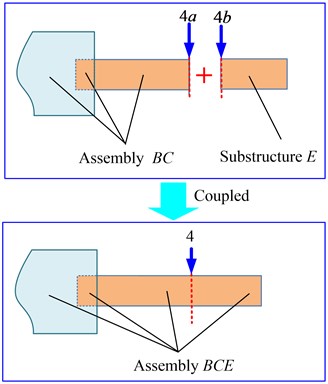
a) Coupling between assembly $B C$ and substructure $E$

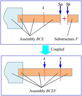
b) Coupling between assembly $B C E$ and substructure $F$

3. Receptance pre-experiment method

If theoretical calculation methods on the coupling of two substructures are used to get the information on the joint interface between the workpiece and the chuck, the receptance coupling model would be established under many hypotheses and simplifications. Which not only lead to tedious calculation formulas, but also the dubious results of contact stiffness, damping and other dynamic parameters. Besides, when the workpiece is under clamped-free boundary condition, its real joint interface is affected by many complex factors, and mishandling or careless treatment with them could easily lead to the rise of calculation error. As the measured FRFs of the workpiece-chuck assembly contain the useful information of the joint interface, here an experimental method is proposed to overcome the limitations in traditional calculation methods, namely “receptance pre-experiment method”. In this method, FRF measurement of a “calibration shaft” inserted in the chuck is combined with some numerical calculations to obtain 2×2 receptance matrix of chuck section, which reflects coupling dynamics between the workpiece and the chuck by the related translational and rotational receptance. Then, according to the prediction principle in section 2, we can employ receptance coupling method to predict FRF of cylindrical workpiece with high precision and efficiency.

3.1. The receptance matrix of chuck section

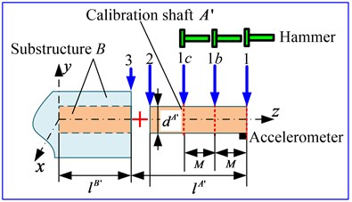
Assume that a calibration shaft $A'$ is installed in the chuck with the free length $l^{A'}$ , clamping length $l^{B'}$ and diameter $d^{A'}$ , and the clamped part of the calibration shaft is still divided into substructure $B$ , as seen in Fig. 6. In order to get the receptance matrix of chuck section, $R_{33}^{B}$ , firstly it is necessary to obtain 2×2 receptance matrix of assembly $A' B$ at cross section 1, $R_{11}^{A' B}$ . Referring to the derivation process of receptance coupling between substructure $B$ and substructure $C$ , replace substructure $C$ with calibration shaft $A'$ in Eq. (13) and cross section 4 $a$ would be replaced by cross section 1, thus $R_{11}^{A' B}$ (or $R_{11}^{B A'}$ ) can be expressed as follow:

25

R_{11}^{A' B} = [\begin{array}{l} H_{11}^{A' B} & L_{11}^{A' B} \\ N_{11}^{A' B} & P_{11}^{A' B} \end{array}] = R_{11}^{A'} - R_{12}^{A^{'}} {(R_{22}^{A^{'}} + R_{33}^{B})}^{- 1} R_{21}^{A^{'}} .

Extract $R_{33}^{B}$ from the right side of Eq. (25), and it can be expressed as follow:

26

R_{33}^{B} = R_{21}^{A'} {(R_{11}^{A'} - R_{11}^{A' B})}^{- 1} R_{12}^{A'} - R_{22}^{A^{'}},

where, $R_{21}^{A'}$ , $R_{11}^{A'}$ , $R_{12}^{A'}$ , $R_{22}^{A'}$ can be calculated by reference to the derivation process of Eq. (1) to Eq. (5), therefore, only $R_{11}^{A' B}$ is still unknown. The following will adopt two FRF measurement techniques to get $R_{11}^{A' B}$ , including two points impact method and three points impact method.

Fig. 6FRFs measurement of the calibration shaft

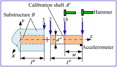
a) Two points impact method

b) Three points impact method

3.1.1. Two points impact method

Two points impact method can be used to obtain $R_{11}^{A' B}$ , when the measured curves of FRF data of the calibration shaft are smooth and the corresponding coherence coefficient is close to 1. Suppose an accelerometer is placed at cross section 1 along the $y$ direction (or $x$ direction), and a fixed impact distance, $M$ , between the cross section 1 and 1 $b$ is chosen to conduct two points impact measurement with the same direction of the accelerometer (the influence of impact distance will be discussed in section 3.2), so that FRFs data of assembly $A' B$ , $H_{11}^{A' B}$ and $H_{11 b}^{A' B}$ , can be obtained. Then, using the first-order finite difference method [16], other translational and rotational receptance, $L_{11}^{A' B}$ , $N_{11}^{A' B}$ , $P_{11}^{A' B}$ can be derived by Eq. (27) and Eq. (28), and through combining these receptances with $H_{11}^{A' B}$ , $R_{11}^{A' B}$ can be also derived by Eq. (29). Finally, substitute Eq. (29) into the Eq. (26), and the 2×2 receptance of chuck section, $R_{33}^{B}$ , can be completely obtained:

27

L_{11}^{A' B} = N_{11}^{A' B} = \frac{H_{11}^{A' B} - H_{11 b}^{A' B}}{M},

28

P_{11}^{A' B} = \frac{L_{11}^{A' B} N_{11}^{A' B}}{H_{11}^{A' B}} = \frac{L_{11}^{A' B^{2}}}{H_{11}^{A' B}} = \frac{{(\frac{H_{11}^{A^{'} B} - H_{11 b}^{A^{'} B}}{M})}^{2}}{H_{11}^{A^{'} B}},

29

R_{11}^{A' B} = [\begin{array}{l} H_{11}^{A' B} & L_{11}^{A' B} \\ N_{11}^{A' B} & P_{11}^{A' B} \end{array}] = [\begin{array}{l} H_{11}^{A' B} & \frac{H_{11}^{A' B} - H_{11 b}^{A' B}}{M} \\ \frac{H_{11}^{A' B} - H_{11 b}^{A' B}}{M} & {(\frac{H_{11}^{A' B} - H_{11 b}^{A' B}}{M})}^{2} / H_{11}^{A' B} \end{array}] .

3.1.2. Three points impact method

If the resulting FRFs of the calibration shaft are not very well due to the interference of background noise, three points impact method can be used as an alternative to obtain $R_{11}^{A' B}$ . Suppose that an accelerometer is placed at cross section 1 along the $y$ direction (or $x$ direction), and a fixed impact distance, $M$ , between the cross section 1, 1 $b$ and 1 $c$ is chosen to conduct three points impact measurement with the same direction of the accelerometer, so that we can obtain FRFs data of assembly $A' B$ , $H_{11}^{A' B}$ , $H_{11 b}^{A' B}$ and $H_{11 c}^{A' B}$ . Similarly, using the second-order finite difference method, $L_{11}^{A' B}$ , $N_{11}^{A' B}$ , $P_{11}^{A' B}$ can also be derived by Eq. (30) and Eq. (31), and through combining these receptances with $H_{11}^{A' B}$ , $R_{11}^{A' B}$ can be derived by Eq. (32). Finally, substitute Eq. (32) into the Eq. (26), and the 2×2 receptance matrix of chuck section, $R_{33}^{B}$ , can be completely obtained:

30

L_{11}^{A' B} = N_{11}^{A' B} = \frac{3 H_{11}^{A' B} - 4 H_{11 b}^{A' B} + H_{11 c}^{A' B}}{2 M},

31

P_{11}^{A' B} = \frac{L_{11}^{A' B} N_{11}^{A' B}}{H_{11}^{A' B}} = \frac{L_{11}^{A' B^{2}}}{H_{11}^{A' B}} = \frac{{(\frac{3 H_{11}^{A^{'} B} - 4 H_{11 b}^{A^{'} B} + H_{11 c}^{A^{'} B}}{2 M})}^{2}}{H_{11}^{A^{'} B}},

32

R_{11}^{A' B} = [\begin{array}{l} H_{11}^{A' B} & L_{11}^{A' B} \\ N_{11}^{A' B} & P_{11}^{A' B} \end{array}] = [\begin{matrix} H_{11}^{A' B} & \frac{3 H_{11}^{A' B} - 4 H_{11 b}^{A' B} + H_{11 c}^{A' B}}{2 M} \\ \frac{3 H_{11}^{A' B} - 4 H_{11 b}^{A' B} + H_{11 c}^{A' B}}{2 M} & \frac{{(\frac{3 H_{11}^{A^{'} B} - 4 H_{11 b}^{A^{'} B} + H_{11 c}^{A^{'} B}}{2 M})}^{2}}{H_{11}^{A^{'} B}} \end{matrix}] .

3.2. Influences on the receptance matrix of chuck section

Successfully obtaining the receptance matrix of chuck section, $R_{33}^{B}$ , is the prerequisite and basis for the prediction of FRF of cylindrical workpiece. In this section, the influences on $R_{33}^{B}$ are experimentally analyzed, so that a practical methodology can be found out to determine: (I) The number of calibration shaft; (II) The free length $l^{A'}$ , clamping length $l^{B'}$ and diameter $d^{A'}$ ; (III) Some techniques which can help improve accuracy of $R_{33}^{B}$ .

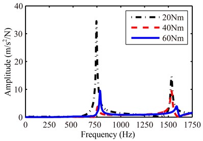
Fig. 7FRFs of the calibration shaft measured at different tightening torque

3.2.1. The real clamping effect of the inserted calibration shaft

Install the calibration shaft into the chuck with $l^{A'} =$ 40 mm, $l^{B'} =$ 80 mm, $d^{A'} =$ 25 mm (these parameters are all measured by vernier caliper for three times and the average is used as test result, and clamping length is indirectly obtained by subtracting free length from the total length), and experimentally obtain FRFs data of the inserted calibration shaft clamped at 20 Nm, 40 Nm and 60 Nm, as seen in Fig. 7.

It can be observed that there is a big difference between each nature frequency as well as the corresponding amplitude under different clamping torque, which will undoubtedly affect the accuracy of $R_{33}^{B}$ . Therefore, in receptance pre-experiment, we must ensure that one end of the calibration shaft be effectively clamped. To this end, a torque wrench is used to determine the level of tightening torque on the square holes of the chuck, and several tests on the first 2 nature frequencies of the calibration shaft need to be conducted. If the resulting nature frequencies between each experiment are close to each other, we will keep using this tightening torque value to finish all of the experiment. If the difference between each nature frequency is big (e.g., more than 10 Hz), we need to increase torque value and to repeat above experiment.

3.2.2. The impact distance

Install and set the calibration shaft with the following parameters, $l^{A'} =$ 120 mm, $l^{B'} =$ 85 mm, $d^{A'} =$ 25 mm. Firstly, make sure it is effectively clamped by lathe chuck. Then, conduct FRF measurement by three points impact method with different impact distance $M$ , namely 20 mm, 40 mm, 60 mm, and Fig. 8 gives the direct and cross FRFs, $H_{11}^{A' B}$ , $H_{11 b}^{A' B}$ and $H_{11 c}^{A' B}$ at the cross section 1, 1 $b$ and 1 $c$ with $M =$ 20 mm. Subsequently, substitute different $M$ into the Eq. (32) and then obtain $R_{33}^{B}$ by Eq. (26), the resulting displacement-to-force receptance $h_{33}^{B}$ can also be extracted, as seen in Fig. 9. It can be observed that impact distance does not have obvious influence on $R_{33}^{B}$ as each coupling frequency with different $M$ is close to each other (receptance amplitude seems to be different, but it can be adjusted by inputting different loss factor).

Fig. 8The measured FRFs at different cross section with impact distance of 20 mm

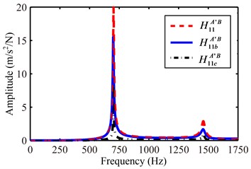
Fig. 9The calculated displacement-to-force receptance of chuck section with different impact distance

3.2.3. Free length of calibration shaft

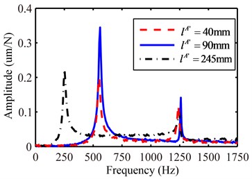
Choose three different calibration shafts with free length $l^{A'} =$ 40, 90, 245 mm and other parameters unchanged ( $l^{B'} =$ 85 mm, $d^{A'} =$ 25 mm). FRF measurement is done within 0-2096 Hz by three points impact method, the resulting FRFs at cross section 1 with different free length are given in Fig. 10. Besides, the corresponding displacement-to-force receptance curves can be obtained, as seen in Fig. 11. It can be observed that free length of the calibration shaft does not have obvious influence on $R_{33}^{B}$ . However, the used free length should not be too long, otherwise the frequency value might be the nature frequency of the calibration shaft itself (e.g., the first nature frequency, about 250 Hz of the calibration shaft with 245 mm, as seen in Fig. 10, which lead to incorrect coupling frequency of 250 Hz in Fig. 11), rather than the desired coupling frequency value, which would be a serious disturbance to $R_{33}^{B}$ . Good practice in our test dictates that the free length $l^{A'}$ should meet the following relation in Eq. (33):

33

\frac{1}{3} L \leq l^{A^{'}} \leq \frac{2}{3} L,

where, $L$ refers to the length of the lathe chuck.

Fig. 10The measured FRFs at cross section 1 with different free length

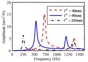
Fig. 11The calculated displacement-to-force receptance of chuck section with different free length

3.2.4. Clamping length of calibration shaft

Choose four different calibration shafts, namely $S_{A}$ , $S_{B}$ , $S_{C}$ , $S_{D}$ with clamping length $l^{B'} =$ 40, 80, 120, 165 mm and other parameters unchanged ( $l^{A'} =$ 80 mm, $d^{A'} =$ 25 mm). Table 1 lists the resulting coupling frequencies of chuck section obtained by receptance pre-experiment method when FRFs of calibration shafts with different clamping length are tested. From which we can found out that the receptance matrix of chuck section, $R_{33}^{B}$ , is closely related to the clamping length of calibration shaft, the frequency values will gradually raise with the increase of $l^{B'}$ , and the first coupling frequency seems to be heavily affected than the second one as the frequency difference between $S_{A}$ and $S_{D}$ reaches to 13.5 % while the second one 6.9 %. In order to improve prediction accuracy of the workpiece by receptance coupling method, we need to establish the relation between $R_{33}^{B}$ and $l^{B'}$ by repeating receptance pre-experiment several times in practice. For instance, get different $R_{33}^{B}$ by increasing $l^{B'}$ at a fixed interval (20 mm or shorter), which may lower prediction efficiency a little bit, but it will allow us to get FRFs of cylindrical workpiece with high precision.

Table 1The first two coupling frequencies of chuck section obtained by receptance pre-experiment method when FRFs of calibration shafts with different clamping length are tested

Type	Clamping length (mm)	Mode 1		Mode 2
Type	Clamping length (mm)	Coupling frequency (Hz)	Frequency difference (%)	Coupling frequency (Hz)	Frequency difference (%)
$S_{A}$	40	503	–	1189	–
$S_{B}$	80	540	7.4	1231	3.5
$S_{C}$	120	564	12.1	1243	4.5
$S_{D}$	165	571	13.5	1271	6.9

3.2.5. Diameter of calibration shaft

Choose several different calibration shafts, namely $S_{E}$ , $S_{F}$ , $S_{G}$ , $S_{H}$ , $S_{I}$ with different diameter ( $d^{A'} =$ 20, 25, 37, 54, 102 mm) and other parameters unchanged ( $l^{B'} =$ 85 mm, $l^{A'} =$ 120 mm) to complete FRF measurement. Table 2 lists the resulting coupling frequencies of the chuck obtained by receptance pre-experiment method when FRFs of calibration shafts with different diameter are tested. It can be found out that the receptance matrix of chuck section $R_{33}^{B}$ is also affected by the diameter of calibration shaft. But frequency difference is within an acceptable range (the max frequency difference between $S_{E}$ and $S_{H}$ is below 5 %, except for the one between $S_{E}$ and $S_{I}$ , which is above 20 % due to the small ratio of length to diameter of $S_{I}$ (it cannot be modeled as an Euler-Bernoulli beam). Therefore, if the ratio of length to diameter of calibration shafts can meet the following relation in Eq. (34), we can basically neglect the influence from the diameter parameter, and use a single calibration shaft to get $R_{33}^{B}$ :

34

\frac{l^{A^{'}}}{d^{A^{'}}} \geq 2.5 ~ 3 .

Table 2The first two coupling frequencies of chuck section obtained by receptance pre-experiment when FRFs of calibration shafts with different diameter are tested

Type	Diameter (mm)	Ratio of length to diameter	Mode 1		Mode 2
Type	Diameter (mm)	Ratio of length to diameter	Coupling frequency (Hz)	Frequency difference (%)	Coupling frequency (Hz)	Frequency difference (%)
$S_{E}$	20	6.0	538	–	1213	–
$S_{F}$	25	4.8	544	1.1	1238	2.1
$S_{G}$	37	3.2	523	–2.8	1203	–0.8
$S_{H}$	44	2.7	517	–3.9	1182	–2.6
$S_{I}$	98	1.2	405	–24.7	1117	–7.9

From the analysis of the above influences, it can be concluded: (I) Only one calibration shaft is needed in the receptance pre-experiment, but this calibration shaft should be effectively clamped by lathe chuck; (II) Receptance matrix of chuck section is mainly affected by clamping length of calibration shaft if its free length and diameter can meet the relation in Eq. (33) and Eq. (34); (III) It is necessary to establish the relation between the receptance matrix of chuck section and clamping length of calibration shaft by repeating receptance pre-experiment several times, so that we can employ receptance coupling method to predict FRF of different workpiece with high precision.

4. Prediction procedure

Combining with the proposed receptance pre-experiment method in section 3, prediction procedure of FRFs of cylindrical workpiece by receptance coupling method can be divided into the following steps.

4.1. Obtain the receptance matrix of the chuck section under certain clamping length of calibration shaft

This step involves four substeps. Firstly, choose an appropriate calibration shaft, whose free length and diameter should meet the relation in Eq. (33) and Eq. (34); then, install the calibration shaft into the chuck with certain clamping length and make sure that one end of the calibration shaft be effectively clamped by the torque wrench; next, obtain FRFs of the calibration shaft by two or three points impact method; finally, obtain the 2×2 receptance matrix of chuck section by finite difference method.

4.2. Establish the relation between the receptance matrix of chuck section and clamping length of calibration shaft

According to the experimental analysis conclusion on the influences of the receptance matrix of chuck section in section 3, it is mainly affected by clamping length of calibration shaft. Therefore, it is necessary to establish the relation between the receptance matrix of chuck section and clamping length of calibration shaft by increasing clamping length at a fixed interval (20 mm or shorter). Thus, for different cylindrical workpiece while its lamping length is close to the one of calibration shaft, its FRFs can be predicted by using the related receptance data already obtained in the receptance pre-experiment.

4.3. Calculate the receptance of cylindrical workpiece

According to the prediction principle in section 2, cylindrical workpiece can be represented by substructure $A$ , which can be simpled as an Euler-Bernoulli beam model with different free length and diameter measured by the vernier caliper. After inputting the specific parameters, such as length, diameter, mass, density, Young’s modulus, Poisson’s ratio, moment of inertia and loss factor (which can be determined by the “half-power bandwidth” calculation on the FRFs data), the direct receptance and cross receptance of the workpiece can be calculated in the free-free state. It should be noted that the mass of the workpiece involved in the calculation is only the free part as its clamped part is already divided into substructure $B$ .

4.4. Predict FRFs of cylindrical workpiece

Use different cross section to divide cylindrical workpiece (substructures $A$ ), to represent different excitation point and response point, and sequentially couple different substructure with lathe chuck (substructures $B$ ) by receptance coupling method. For direct FRF prediction of the workpiece, extract the displacement-to-force receptance from Eq. (19), and for cross FRF prediction, extract the displacement-to-force receptance from Eq. (24).

5. Experimental verification

In this section, a stepped cylindrical workpiece, whose dimensions and mass parameters is listed in Table 3, is installed into the chuck of CAK3675 CNC lathe with tightening torque of 60 Nm on its square holes, as seen in Fig. 12. It is composed of #45 steel with Young’s modulus of 2×10¹¹ Pa, Poisson’s ratio of 0.3, and the density of 7800 kg/m3. FRF measurement system is set up to experimentally measure the workpiece’s direct and cross FRF, and these measured FRFs are used to verify the predicted results.

Table 3Dimensional and mass parameters of stepped cylindrical workpiece

Clamping length	Step-I			Step-II
Clamping length	Free length (mm)	Diameter (mm)	Mass (g)	Free length (mm)	Diameter (mm)	Mass (g)
85	35	20	85.8	105	15	144.7

5.1. FRF measurement system

Fig. 12 shows the schematic of FRF measurement system of cylindrical workpiece, The pulse excitation is provided by a hammer (BK 8206-002) and response signal is measured by lightweight accelerometer, BK4517 of mass 0.6 g (to avoid the errors due to the additional mass and stiffness by contact measurement). BK PULSE 3560D Mobile Front-End is used to record excitation and response signals, PULSE LabShop software, version 12.6, is used to control the data acquisition. Besides, Dell notebook computer (with Intel Core i7 2.93 GHz processor and 4G RAM) is used to operate PULSE LabShop software and store measured data.

5.2. Verification procedure and results

On the one hand, FRFs data of stepped cylindrical workpiece with the clamping length of 85 mm is measured by impact testing within 0-3200 Hz. The accelerometer is attached firmly by 3 M adhesive tape on the free end (cross section 1) of the measured workpiece along the $x$ direction, and two different excitation points are chosen to be knocked by the hammer, one is at cross section 1, the other is at cross section 1 $c$ (the distance between them is about 40 mm). PULSE LabShop software takes excitation signal and response signal and conducts FFT to convert the data to the frequency domain, and numerical integration technique (Simpson) is adopted to convert acceleration to displacement, so that the output is the desired FRFs curve (amplitude of displacement-to-force versus frequency). The measured direct and cross FRF of stepped cylindrical workpiece along the $x$ direction can be seen in Fig. 13(a) and Fig. 13(b), and finishing the experiment takes about 1-2 minutes, yet time cost in installing and clamping the measured workpiece into the chuck is high (about 3-5 minutes), so the total measurement time is about 4-7 minutes.

Fig. 12Schematic of FRF measurement system of cylindrical workpiece of CNC lathe

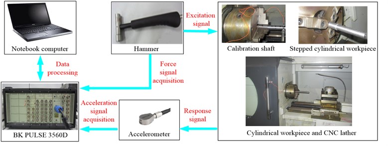
Fig. 13The measured and predicted FRFs of stepped cylindrical workpiece along the x direction

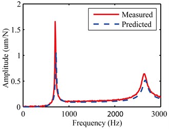
a) Direct FRF curve

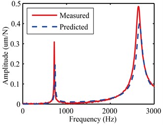
b) Cross FRF curve

On the other hand, FRFs data of stepped cylindrical workpiece is predicted in accordance with the prediction procedure proposed in section 4. Firstly, choose an appropriate calibration shaft $A'$ (with free length $l^{A'} =$ 120 mm and diameter $d^{A'} =$ 25 mm, which could meet the relation in Eq. (33) and Eq. (34)) and carry out FRF measurement by three points impact method. Then, obtain the required 2×2 receptance matrix of chuck section $R_{33}^{B}$ under different clamping length. Next, choose clamping length $l^{B'} =$ 85 mm and the related $R_{33}^{B}$ , and couple $R_{33}^{B}$ with the calculated receptance, such as $R_{j k}^{C}$ , $R_{j k}^{B C}$ , $R_{j k}^{D}$ , $R_{j k}^{B C D}$ , $R_{j k}^{B C E}$ , $R_{j k}^{B C E F}$ ( $j$ , $k$ denote different cross section), which can be obtained by dividing the workpiece (substructure $A$ ) into different substructure $C$ , $D$ , $E$ , $F$ with cross section 1 and 1 $c$ . Finally, the predicted direct and cross FRF of stepped cylindrical workpiece along the $x$ direction can be obtained by extracting the displacement-to-force receptance from Eq. (19) and Eq. (24), which are also plotted in Fig. 13(a) and Fig. 13(b) respectively. The related calculation program has already been realized by MATLAB, it takes about 1 minute to input the required dimensions, material and damping parameters, and the total calculation time is less than 20 seconds, which is an obvious reduction in time costs than experimental method.

5.3. Result analysis

As can be seen from Fig. 13, the overall agreement between the predicted and measured FRFs of stepped cylindrical workpiece is good. Thus, practicability and effectiveness of receptance coupling method have been demonstrated. However, small deviations are also seen, the possible reasons are: (I) Calculation error in loss factor due to the complexity of damping characteristics, which lead to amplitude differences of FRF curves; (II) Inaccurate dimensional and mass parameter of the workpiece as well as calibration shaft resulted from test error; (III) Deviations and uncertainties in joint interface between the workpiece and chuck.

6. Conclusions

In this research, receptance coupling method is applied in the analytic prediction of FRFs of cylindrical workpiece in CNC lathe, and its practicability and efficiency have been demonstrated. In order to improve prediction accuracy, receptance pre-experiment method is proposed to obtain 2×2 receptance matrix of chuck section which represents the most crucial coupling receptance of the workpiece-chuck assembly.

Some major influences on the receptance matrix of chuck section are experimentally analyzed, and it has been found that: (I) Only one calibration shaft is needed in the receptance pre-experiment, but this calibration shaft should be effectively clamped by lathe chuck; (II) Receptance matrix of chuck section is mainly affected by clamping length of calibration shaft; (III) It is necessary to establish the relation between the receptance matrix of chuck section and clamping length of calibration shaft, so that receptance coupling method can be used to predict FRF of different workpiece with high precision.

References

Faassen R. P. H., van de Wouw N., Oosterling J. A. J., Nijmeijer H. Prediction of regenerative chatter by modelling and analysis of high-speed milling. International Journal of Machine Tools and Manufacture, Vol. 43, Issue 14, 2003, p. 1437-1446.

Search CrossRef
Lin R. M., Zhu J. Model updating of damped structures using FRF data. Mechanical Systems and Signal Processing, Vol. 20, Issue 8, 2006, p. 2200-2218.

Search CrossRef
Sun X. H., Zhang L. M., Wang T. Noise reduction of frequency response function using singular value decomposition. Journal of Vibration, Measurement and Diagnosis, Vol. 29, Issue 3, 2009, p. 325-328.

Search CrossRef
Bishop R. E. D., Johnson D. C. The Mechanics of Vibration. Cambridge University Press, London, 1960.

Search CrossRef
Schmitz T. L., Donaldson R. R. Predicting high-speed machining dynamics by substructure Analysis. Annals of the CIRP, Vol. 49, Issue 1, 2000, p. 303-308.

Search CrossRef
Schmitz T. L., Davies M. A., Kennedy M. D. Tool point frequency response prediction for high-speed machining by RCSA. Journal of Manufacturing Science and Engineering, Vol. 123, Issue 4, 2001, p. 700-707.

Search CrossRef
Schmitz T. L., Duncan G. S. Receptance coupling for dynamic prediction of assemblies with coincident neutral axes. Journal of Sound and Vibration, Vol. 289, Issue 4, 2006, p. 1045-1065.

Search CrossRef
Schmitz T. L., Powell K., Won D., et al. Shrink fit tool holder connection stiffness/damping modeling for frequency response prediction in milling, Part 1: receptance model. Proceedings of the Second CIRP-HPC 2006, Vancouver, Canada, 2006.

Search CrossRef
Schmitz T. L., Powell K., Won D., et al. Shrink fit tool holder connection stiffness/damping modeling for frequency response prediction in milling, Part 2: finite element model. Proceedings of the Second CIRP-HPC 2006, Vancouver, Canada, 2006.

Search CrossRef
Schmitz T. L., Davies M. A., Medicus K., Snyder J. Improving high-speed machining material removal rates by rapid dynamic analysis. Annals of the CRIP, Vol. 50, Issue 1, 2001, p. 263-268.

Search CrossRef
Park S. S., Altintas Y., Movahhedy M. Y. Receptance coupling for end mills. International Journal of Machine Tools and Manufacture, Vol. 43, Issue 9, 2003, p. 889-896.

Search CrossRef
Erturka A., Ozguvena H. N., Budak E. Analytical modeling of spindle-tool dynamics on machine tools using Timoshenko beam model and receptance coupling for the predict ion of tool point FRF. International Journal of Machine Tools and Manufacture, Vol. 46, Issue 15, 2006, p. 1901-1912.

Search CrossRef
Ahmadi K., Ahmadian H. Modelling machine tool dynamics using a distributed parameter tool-holder joint interface. International Journal of Machine Tools and Manufacture, Vol. 47, Issue 12, 2007, p. 1916-1928.

Search CrossRef
Zhang J., Schmitz T. L., Zhao W. H., Lu B. H. Receptance coupling for tool point dynamics prediction on machine tools. Chinese Journal of Mechanical Engineering-English Edition, Vol. 24, Issue 3, 2011, p. 340-345.

Search CrossRef
Catania G., Mancinelli N. Theoretical-experimental modeling of milling machines for the prediction of chatter vibration. International Journal of Machine Tools and Manufacture, Vol. 51, Issue 4, 2011, p. 339-348.

Search CrossRef
Press W. H. Numerical Recipes 3rd Edition: the Art of Scientific Computing. Cambridge University Press, London, 2007.

Search CrossRef

About this article

Received

29 May 2014

Accepted

11 April 2015

Published

30 June 2015

SUBJECTS

Mechanical vibrations and applications

Keywords

frequency response function

receptance pre-experiment method

receptance coupling

cylindrical workpiece

Acknowledgements

This study was supported by the National Key Scientific Instrument and Equipment Development Project of China granted No. 2013YQ470765; the National Natural Science Foundation of China granted No. 51375079; the National Basic Research Program of China granted No. 2011CB706504.

This is an open access article distributed under the Creative Commons Attribution License, which permits unrestricted use, distribution, and reproduction in any medium, provided the original work is properly cited.