Application of unsupervised identification of dissolved gases in transformer oil based on spin coating film making process

1. Introduction

In electrical systems, these devices fulfill a key role in voltage conversion, isolation, and compliance regulation. Problems such as aging and damage of insulation materials, long-term overload and overheating, iron core failure, etc. can all lead to power system paralysis. Advanced fault diagnosis technology can detect potential problems before a fault occurs, realize the transformation from traditional passive maintenance to active preventive maintenance, and greatly reduce power outage losses and maintenance costs caused by sudden faults.

Collecting and assessing volatiles in transformer fluid is one of the key approaches for monitoring the condition and diagnosing faults in power system transformers. Oil and gas separation membrane technology is a technique for reliably isolating volatiles from transformer fluid. Oil and gas separation membranes generally consist of two parts: a separation layer and a support layer. Among them, the separation layer is usually composed of oleophobic polymer materials, which are responsible for isolating the penetration of insulating oil. Due to thermal motion, gas molecules within the fluid will move into the separation layer and gradually spread to the support layer. Therefore, the thinner the separation layer and the higher the free volume fraction of the membrane material, the shorter the gas diffusion time and the higher the gas extraction efficiency. The support layer is usually composed of porous material, which is responsible for carrying the separation layer and providing some structural strength. The pore size and void ratio of porous materials greatly affect the film-forming quality of the separation layer and the gas transmission rate inside it. Although a larger pore size in the support layer is beneficial to the diffusion of gas, when the separation layer is coated, it will easily cause the separation layer solution to penetrate into the pores and increase the penetration time of the gas in the separation layer. If the pore size of the support layer is small, it will affect the diffusion rate of gas inside it. The traditional dip coating method will improve the above problems by controlling the dip coating time and pulling speed, but it still faces problems such as difficult to control film parameters and uneven film thickness [1].

To more accurately describe fault categories, fault identification technology distinguishes different fault types by extracting features from data. However, traditional identification methods, such as algorithms based on threshold settings, lack flexibility and adaptability to complex patterns, making it difficult to maintain stable performance [2]-[3]. To address these issues, researchers have proposed various optimized methods, including the use of classic machine learning techniques like support vector machines (SVM) [4]-[5], random forests, as well as introducing deep learning models such as convolutional neural networks (CNN) and long short-term memory networks (LSTM) [6]-[7]. These methods have improved diagnostic accuracy but also brought new challenges. On one hand, traditional methods perform limitedly when handling nonlinear data; on the other hand, deep learning models offer higher performance but require large volumes of high-quality labeled data. Especially for dissolved gases in oil, the data in practical applications are often sparsely labeled or completely unlabeled [8], posing strict requirements for training and storage. Therefore, avoiding overfitting and enhancing model generalization ability under data scarcity has become a critical research direction. Additionally, the generation mechanism of dissolved gas cases in oil and its optimization in an unsupervised learning environment must be considered [9].

Despite the success of existing sample expansion algorithms, such as GANs based on image recognition, in certain domains, they encounter numerous limitations when applied to dissolved gases in oil. For example, ACGAN overcomes data non-stationarity by generating samples, improving diagnostic classification accuracy [11] and effectively addressing noise contamination and few fault samples in vibration signals; integrating stacked denoising autoencoders into GAN can transform one-dimensional fault sequences into two-dimensional grayscale images and use CGAN to generate grayscale image samples, addressing fault diagnosis needs under sample imbalance [12]-[13]; combining RNN with CNN batch normalization, transfer learning, and three-element representation diagrams has also enhanced the effectiveness of sample identification models [14]. Although these methods have achieved certain successes in improving diagnostic performance, they still face issues of poor stability. Notably, CNN models originate from the field of image processing and excel at image generation tasks, whereas the dissolved gas sequences in oil are highly variable and diverse discrete data types. Therefore, applying GAN-like neural networks directly to generate such dissolved gas data may result in problems such as repeated samples, suboptimal generation efficiency, and unsatisfactory overall outcomes. For discrete sequence expansion, studies have proposed methods like amplitude compression, dynamic inversion, sequence EEMD decomposition expansion, among others [15]-[16]. While these methods increase inter-category differences, they primarily suit non-stationary data. Concerning the distinctiveness of dissolved gas parameters in transformer oil, the expansion process can lead to changes in data labels, affecting the reliability of diagnostic results.

Simultaneously, research on unsupervised case identification of dissolved gases in oil is relatively scarce. For small-sample recognition problems of other types of data, studies have proposed a comprehensive framework composed of a Pseudo Label Extraction (PLE) module and a Reconstruction Error-based Anomaly Detection (READ) module. This framework first assigns pseudo-labels to the data using DBSCAN's adaptive pseudo-label extraction algorithm, then extracts multi-level temporal features and calculates reconstruction errors through a dual LSTM autoencoder. Finally, it trains a logistic regression classification model using pseudo-labels to classify the reconstruction errors for anomaly detection [17]. Additionally, there are studies that have improved the traditional Time-series Generative Adversarial Network (TimeGAN) architecture based on a least squares decision loss function, achieving precise identification of perturbation sequences in environments with no or few labels [18]. These studies provide valuable experience in addressing the challenges of small sample sizes and unlabeled data; however, further exploration and innovation are still required for the specific application scenarios of dissolved gases in oil, especially in dealing with insufficient data labeling and sample imbalance issues.

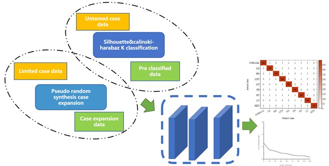
On the one hand, this article will explore a film-making process based on spin coating. The spin-coating method is not only easier to control the film-making process parameters, but also can better inhibit the penetration of the separation layer solution into the pores due to the introduction of centrifugal force, thereby producing thinner films. The separation layer can improve the degassing efficiency and thereby improve the collection efficiency of dissolved gas cases; on the other hand, in order to solve the problems of how to accurately classify case faults under unsupervised operation and how to effectively expand the cases of dissolved gases in oil, this paper uses K-means++ clustering The method identifies characteristics of dissolved gas instances in oil and introduces a K value estimation technique utilizing silhouette score and Calinski-Harabaz index for pre-classifying unlabeled data. Afterwards, some samples of each category can be marked to which they belong. The labels can be used without labeling one by one; Through examining the similarities between the volatiles sequences in transformer fluid and DNA sequences, a pseudo-random integration technology is introduced to boost the volatiles content in transformer fluid, increasing the number of gas instances, thereby providing more training data. Furthermore, this approach can also lessen the instability of classification precision due to randomness; finally, based on the Gaussian multi-classification model, a pre-classification, re-expansion, and post-classification classification Strategies to realize transformer fault identification.

2. Preparation of oil and gas separation membrane

Fluid and vapor separation membranes typically include two main components: the separation layer and the support layer. The separation layer primarily employs oleophobic polymer materials, which serve to block the insulating fluid while permitting volatiles to permeate and diffuse to the support layer due to thermal motion. Therefore, the thinner the separation layer and the higher the free volume fraction of the membrane material, the faster the gas molecules can be separated from the oil, thereby increasing the degassing efficiency. The support layer is generally made of porous materials. It not only provides the necessary structural strength for the separation layer, but also affects the film-forming quality of the entire membrane and the gas transmission rate within the membrane. The selection of the pore size and porosity of the support layer is very critical; if the pore size is too large, it will easily cause the solution to penetrate into the pores when coating the separation layer, increasing the time for the gas to pass through the separation layer; conversely, if the pore size is too small, it may limit the Effective diffusion of gas within the support layer.

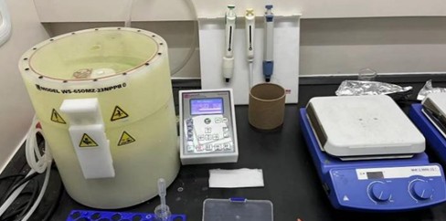
The introduction of a new technique involving spin coating aims to enhance the manufacturing process of oil and gas separation membranes. The spin coating method has better controllability, and the film thickness can be easily adjusted by adjusting conditions such as rotation speed. More importantly, due to the effect of centrifugal force, this method can effectively prevent the separation layer material from penetrating into the pores of the support layer, helping to form a thinner and more uniform separation layer, thereby significantly improving the degassing performance. Fig. 1 shows a schematic diagram of the membrane production platform developed based on this technology, further demonstrating how this method can achieve efficient and stable production of fluid and vapor separation membranes.

To further illustrate the efficient and stable production process of oil and gas separation membranes using the spin coating method, Fig. 1 provides a schematic diagram of the membrane production platform developed based on this technology. The experimental setup consists of several key components: a spin coater, ceramic support layer, spin coating solution supply system, constant temperature drying oven, and parameter adjustment equipment for precise control of film thickness.

The detailed workflow of the experimental setup is as follows: Preparation of Ceramic Support Layer: Initially, the ceramic support layer is soaked in 95 % anhydrous ethanol and cleaned in an ultrasonic cleaning machine for 10 minutes. It is then dried at 120°C for 2 hours in a constant temperature drying oven. Spin Coating Solution Preparation: A uniform spin coating solution is prepared using the AF2400 separation layer material. Spin Coating Process: The ceramic layer with a pore size of 100 nm is adsorbed upward on the vacuum suction cup of the spin coater. In the first stage, the spin coater's rotation speed is set to 800 rpm for 20 seconds. During this period, an appropriate volume of AF2400 solution is slowly and evenly dropped onto the surface of the ceramic base film using a pipette. In the second stage, the rotation speed is increased to 1200 rpm for 1 minute to ensure the solution is uniformly coated on the ceramic surface. Drying and Curing: After spin-coating, the ceramic is removed from the spin coater and placed in a constant temperature drying oven. It is gradually heated to 245 °C and left for 1 hour to allow the solvent to completely evaporate. Repetition and Storage: The above steps are repeated once, and the prepared oil and gas separation membrane is stored in a clean room under sealed conditions.

Through this detailed experimental setup, we can achieve efficient production of fluid and vapor separation membranes while ensuring their consistent performance and reliability.

Fig. 1Experimental setup for preparing hydrocarbon vapor separation membranes utilizing spin coating

In order to further inhibit the separation layer solution from penetrating into the support layer, this paper uses a double-layer ceramic composite with a pore size of 100/500 nm as the support layer, with thicknesses of 10 μm and 2 mm respectively. The ceramic layer with a pore size of 100 nm and 10 μm can increase the penetration resistance of the solution in the separation layer without significantly increasing the diffusion time of gas in the support layer. It is an ideal structure as a support layer for oil and gas separation membranes. Therefore, this article will use a double-layer composite ceramic with a diameter of 4.0 cm as the support layer and AF2400 as the separation layer to prepare an oil and gas separation membrane.

The main equipment and materials used are shown in Table 1. The preparation process is as follows: a) Soak the ceramics in 95 % anhydrous ethanol and clean them in an ultrasonic cleaning machine for 10 minutes; b) Place the cleaned ceramics in a constant temperature drying oven. Within, dry at 120 °C for 2 hours; c) Adsorb the ceramic layer with a pore size of 100 nm upward on the vacuum suction cup of the uniform spin coater to prepare the spin coating solution; d) Set the rotation speed of the first stage of the uniform spin coater to 800 rpm, time 20 s. During this process, use a pipette to absorb an appropriate volume of AF2400 solution, and drop it evenly and slowly on the surface of the ceramic base film; e) Set the second stage speed of the uniform spin coater to 1200 rpm, time 1 minute , wait for the solution to be evenly coated on the ceramic surface; f) Remove the ceramic after spin-coating the AF2400 solution, place it in a constant temperature drying oven and slowly heat it to 245 °C and leave it for 1 hour to wait for the solvent to completely evaporate; g) Repeat c - f This step is performed once, and the coated oil and gas separation membrane is placed in a clean room for sealed storage.

3. Silhouette-Calinski-Harabaz-K classification

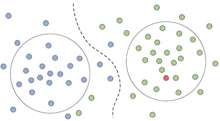
The existing dissolved gas data in oil all contain H2, CH4, C2H2, C2H4, C2H6, CO, CO2 content 7 characteristics, the collected data itself is often Most of the case data collected when the transformer is in an unknown or uncertain state is quantified without labels, and quantitative clustering through manual labeling is too cumbersome. To this end, this article first performs adaptive pre-clustering on limited unlabeled data, as shown in Fig. 2. Afterwards, the labels to which some samples of each category belong can be marked without the need to mark the whole one by one.

Fig. 2Case clustering

An extensively applied unsupervised clustering approach, K-means clustering can automatically group multiple data sequences into K clusters [19]. The placement of the starting cluster centers impacts the effectiveness of the K-means algorithm. Conventional random initialization might lead to inconsistent results. To solve this problem, the K-means++ method selects the sample with the most different characteristics as the initial cluster center, thereby improving the consistency of the clustering algorithm. This paper selects this algorithm as a pre-classification method for cases of dissolved gases in limited oil. The desired number of clusters, an essential input for the K-means++ algorithm, directly influences the set of transformer fault categories identified, thereby significantly affecting the effectiveness of unlabeled samples [20]. Therefore, the problem of $K$ value estimation needs to be solved urgently. Accordingly, an approach for estimating the $K$ value using the Silhouette coefficient and Calinski-Harabaz index is presented [21-22].

The Silhouette coefficient provides an internal measure for evaluating clustering results without needing labeled data. Typically, effective clustering should exhibit high similarity among samples within each group and significant dissimilarity across different groups. In calculating the Silhouette coefficient, similarity and distinction are assessed using within-cluster and between-cluster distances, as illustrated in Eqs. (1-3):

where, $D_i$ denotes the $i$-th instance in group $D_k$, $SC\left(i\right)$ and $S{C}_0$ represents $D_i$ and the Silhouette score of the entire dataset respectively, $\mathrm{d}\mathrm{i}\mathrm{s}{\mathrm{t}}_{\mathrm{i}\mathrm{n}\mathrm{t}\mathrm{r}\mathrm{a}}\left(i\right)$ indicating the relationship between $D_i$ and other instances in the same category. $\mathrm{d}\mathrm{i}\mathrm{s}{\mathrm{t}}_{\mathrm{i}\mathrm{n}\mathrm{t}\mathrm{e}\mathrm{r}}\left(i\right)$ indicating the mean distance from $D_i$ to all instances in the closest adjacent group, and $\mathrm{c}\mathrm{a}\mathrm{r}\mathrm{d}\left({\stackrel{-}{D}}_l\right)$ represents the cardinality of $D_l$. Clearly, the Silhouette coefficient ranges between –1 and 1, and greater values indicate closer within-group proximity and greater separation between groups, reflecting superior clustering performance.

Calinski-Harabaz Index: as another internal evaluation indicator. However, unlike the Silhouette coefficient, which relies on within-cluster and between-cluster distances, the Calinski-Harabaz index uses within-cluster and between-cluster scatter matrices to assess similarity and distinction, and evaluates cluster performance by computing their ratio, serving as a Eq. (4) means:

where $CH$ is the Calinski-Harabaz index, $S{M}_{\mathrm{i}\mathrm{n}\mathrm{t}\mathrm{r}\mathrm{a}}$ and $S{M}_{\mathrm{i}\mathrm{n}\mathrm{t}\mathrm{e}\mathrm{r}}$ represents the scatter matrix of samples within clusters and between clusters respectively, ${C^{\text{'}}}_k$ represents the mean of the sample, and $C_0^{\text{'}}$ represents the average of the entire sample. Likewise, a higher Calinski-Harabaz index indicates better clustering performance.

Given that the features derived from known transformer fault categories are clearly separable, it is reasonable to expect the K-means++ algorithm to perform optimally when $K$ corresponds to the count of fault categories. Building on this premise, this paper can evaluate the output clusters using different $K$ values and select the cluster with the optimal score. Particularly, let $\left[K_0,\mathrm{}{K}_0+1,\mathrm{}...,\mathrm{}{K}_0+\kappa -1\right]$ denote the search range of $K$. Then, compute the performance metric vector s for each grouping outcome with varying $K$. The calculation can be expressed by Eq. (5):

Among them, ${\mathbf{s}}_{SC}$, ${\mathbf{s}}_{CH}$and $\mathbf{s}$ are $1\times \kappa$ arrays, each denoting the Silhouette value, Calinski-Harabaz index and the ultimate performance metric for the grouping outcomes within the specified interval. $\mathbf{s}$ represents the average of the normalized Silhouette scores and the Calinski-Harabaz index, not only scales the ultimate score to [0, 1], enhancing flexibility and reliability compared with using a single measure. Thus, a precise estimate for the category count is achieved, enhancing the dependability and safety of preliminary classification.

4. Case expansion of pseudo-random integration

Random integration initially emerged in genetic engineering and is the foundation of transgenic technologies. Introducing exogenous deoxyribonucleic acid (DNA) into a recipient leads to simultaneous and random insertion into the host genome. Transgenic technology alongside unpredictable incorporation limits the gene integration efficiency of transgenic animals and the genetic stability of target genes [23]. In contrast, in case augmentation, this integrated randomness can be used for data augmentation [24].

There is a certain similarity between the concentration sequence regarding gases suspended in oil and the DNA sequence. Both sequences can be viewed as one-dimensional ordered data streams. Changes in concentration or location will affect the meaning of sample tags or data. The traditional approach is to randomly interchange portions of data from two instances. When used alone, it may cause numerical distortion of some parameters, which may be mistaken for new features by subsequent identification methods. Given that collected dissolved gas in oil case parameters are not perfectly correlated, this treatment may alter the label of the original sample. Therefore, using coherent or incoherent data integration methods to deal with gas parameter cases can replace the traditional random insertion method, which can avoid concentration mutations and keep sample labels unchanged. Generating additional sample cases through random integration is a feasible data augmentation strategy. Its expression is as follows:

where $D_{r{i}_n}$ is the source sample, $D_{ai}$ is the created sample, and $N$ indicates the number of samples chosen for one integration. $M$ denotes the number of initial samples, then the maximum count of distinct instances of $C_M^N$ that case expansion can generate. When $N$ has a reasonable value, $C_M^N$ can be much larger than M. For example, this article assumes $M=$120, $N=$5, $C_M^N=$ 190578024.

However, random integration can boost identification accuracy to some extent, but when the amplitude fluctuation is large, that is, when the level difference of gas parameters dissolved in the fluid is too large, the identification results show significant inaccuracy. This volatility results from the randomness in the case selection process, causing some original samples to be selected far more frequently than others. To minimize the unpredictability introduced by this arbitrary picking, the study introduces a quasi-stochastic integration approach. This strategy divides the integration process into multiple stages, and each stage generates $K$ samples. The calculation method is as shown in Eq. (7):

where [$M$/$N$] indicates the integer part function, signifying downward rounding.

First, $N$ examples are selected from the original data set for integration. Next, after each integration, these selected samples will be removed from the augmented data set, which ensures that each sample is used at most once during the entire round. When the remaining samples in the augmented dataset are insufficient to support further integration, the augmented dataset is reloaded and a new cycle begins. This process continues until the required number of samples is reached. The distinction from purely random integration lies in excluding chosen instances and periodically refreshing the augmented dataset. This optimized cycle selection mechanism reduces the randomness of sample selection, thereby improving the accuracy and stability of identification.

5. GPMC model

Because of the diverse transformer issues, fault diagnosis utilizing the Gaussian process model necessitates multiple-category classification, and multiple-category classification fundamentally constitutes an extension of binary classification.

5.1. Gaussian binary classification

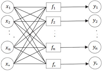
Kernel techniques have received extensive attention in machine learning for extracting data features and are efficiently utilized in SVM and Gaussian process classification models (GPC). Gaussian process (GP) is portrayed as the randomness of combinations of random variables. The classification model computes the likelihood $p\left(x,y\right)$, where $y$ signifies the category tag for two-category classification. Fig. 3 illustrates the GPC model architecture: an implicit function f is employed to transform input values onto the [0,1] interval; the distribution of the implicit function is utilized to determine the class likelihood, that is $\pi \left(x_{*}\right)=p(y_{*}=1|f_{*})$, given a set of data points: $D=(X,y)=\left\{\right(x_i,y_i\left)\right|i=\mathrm{1,2},...,n\}$, $X=\left\{x_i\right|i=\mathrm{1,2},...,n\}$, $n$ represents the extent of sample data, sigmoid functions (including logistic and normal inverse distribution functions) are usually used to “activate” the obtained concealed variable distribution while the class labels are treated as independent variables and Bernoulli distributions. Therefore, the label likelihood probability of each target class is Eq. (8):

8

$p\left(y|\mathbf{f}\right)=\prod _{i=1}^{n}p\left(y_i|f_i\right)=\prod _{i=1}^n\sigma \left(y_i{f}_i\right).$

Among them, $\mathbf{f}=\left\{f_i\right|i=\mathrm{1,2},\dots ,n\}$, $f_i=f\left(x_i\right)\text{.}$ assuming that fi follows a Gaussian distribution, the initial probability of the hidden function can be depicted as Eq. (9):

9

$p\left(\mathbf{f}|X\right)=N\left(\mathbf{f}|\mathbf{\mu },\mathbf{K}\right).$

In which $\mathbf{\mu }$ and $\mathbf{K}$ denote the mean vector and positive covariance matrix, respectively. According to Bayes’ theorem, the posterior probability can be determined Eq. (10):

10

$p\left(\mathbf{f}|y,X,\mathbf{\theta }\right)=\frac{p\left(y|\mathbf{f}\right)p\left(\mathbf{f}|X\right)}{p\left(y|X,\mathbf{\theta }\right)}=\frac{N\left(\mathbf{f}∣0,\mathbf{K}\right)}{p\left(y∣X,\mathbf{\theta }\right)}\prod _{i=1}^n\sigma \left(y_i{f}_i\right),$

where $\mathbf{\theta }$represents the hyperparameters used to parameterize the GP prior. However, in order to categorize the fresh input information $x_{\mathrm{*}}$, the probability distribution of the underlying function needs to be calculated as Eq. (11):

11

$p\left(f_{\mathrm{*}}|x_{\mathrm{*}},y,X,\mathbf{\theta }\right)=\int p\left(f_{\mathrm{*}}|\mathbf{f},x_{\mathrm{*}},X,\mathbf{\theta }\right)p\left(\mathbf{f}|y,X,\mathbf{\theta }\right)d\mathbf{f}.$

The category classification likelihood of incoming test information $x_{\mathrm{*}}$ is derived according to Eq. (12):

12

$p\left(y_{\mathrm{*}}|x_{\mathrm{*}},y,X,\theta \right)=\int \sigma \left(y_{\mathrm{*}}{f}_{\mathrm{*}}\right)p\left(f_{\mathrm{*}}|x_{\mathrm{*}},y,X,\theta \right)d{f}_{\mathrm{*}}.$

Fig. 3GPC classification process: fdenotes the latent function, the input and output of the layers are the data and output class labels. Respectively, y* is the predicted category for test instance x*

However, the distribution in Eq. (8) $p\left(y\right|\mathbf{f})$ is non-Gaussian and the analytical result of the sum potential function distribution in Eq. (11) $p\left(y\right|X,\mathbf{\theta })$ cannot be obtained. Thus, this study employs the Laplace approximation technique to achieve the $q\left(\mathbf{f}\right|y,X,\mathbf{\theta })$ Gaussian distribution and approximate it with the posterior distribution $p\left(\mathbf{f}\right|y,X,\mathbf{\theta })$. The logarithmic posterior probability is defined as $\mathrm{\Psi }\left(\mathbf{f}\right)=\mathrm{l}\mathrm{o}\mathrm{g}p\left(\mathbf{f}\right|y,X,\mathbf{\theta })$, and its calculation is Eq. (13):

13

$\mathrm{\Psi }\left(\mathbf{f}\right)=\mathrm{l}\mathrm{o}\mathrm{g}p\left(y|\mathbf{f}\right)+\mathrm{l}\mathrm{o}\mathrm{g}p\left(\mathbf{f}|X\right)=\mathrm{l}\mathrm{o}\mathrm{g}p\left(y|\mathbf{f}\right)-\frac{1}{2}{\mathbf{f}}^T{\mathbf{K}}^{-1}\mathbf{f}-\frac{1}{2}\mathrm{l}\mathrm{o}\mathrm{g}\left|\mathbf{K}\right|-\frac{n}{2}\mathrm{l}\mathrm{o}\mathrm{g}\left(2\pi \right).$

The $p\left(\mathbf{f}\right|y,X,\mathbf{\theta })$ approximate value of is derived from the Taylor expansion as Eq. (14):

14

$\mathrm{l}\mathrm{o}\mathrm{g}p\left(y\right|X,\mathbf{\theta })=\mathrm{l}\mathrm{o}\mathrm{g}\int \mathrm{e}\mathrm{x}\mathrm{p}(\mathrm{\Psi }\left(\mathbf{f}\right))d\mathbf{f}=\mathrm{l}\mathrm{o}\mathrm{g}p(y\left|\widehat{\mathbf{f}}\right)-\frac{1}{2}{\widehat{\mathbf{f}}}^T{\mathbf{K}}^{-1}\widehat{\mathbf{f}}-\frac{1}{2}\mathrm{l}\mathrm{o}\mathrm{g}\left|\mathbf{B}\right|.$

Among them $\mathbf{B}=\mathbf{K}\cdot ({\mathbf{K}}^{-1}+\mathbf{W})=\mathbf{I}+\mathbf{K}\mathbf{W}$, $\widehat{\mathbf{f}}=\mathrm{a}\mathrm{r}\mathrm{g}\mathrm{m}\mathrm{a}{\mathrm{x}}_{\mathbf{f}}\mathrm{\Psi }\left(\mathbf{f}\right)$, and the hyper parameters are 𝜽 obtained by optimizing using the conjugate gradient technique $\mathrm{l}\mathrm{o}\mathrm{g}p\left(y\right|X,\mathbf{\theta })$. By obtaining the Gaussian approximation of the posterior, the mean and covariance of $f_{\mathrm{*}}$ can be determined. Thus, for the test data $x_{\mathrm{*}}$, the potential distribution term in Eq. (11) can be characterized as Eq. (15), the category classification likelihood is calculated by Eq. (16):

15

$p\left(f_{\mathrm{*}}\right|\mathbf{f},x_{\mathrm{*}},X,\mathbf{\theta })=N(k_{*}^T{\mathbf{K}}^{-1}\widehat{\mathbf{f}},k_{**}-k_{*}^T\left(\mathbf{K}+{\mathbf{W}}^{-1}{)}^{-1}{k}_{*}\right),$

16

$\pi \left(f_{\mathrm{*}}\right)=\int \sigma \left(f_{\mathrm{*}}\right)q\left(f_{\mathrm{*}}|x_{\mathrm{*}},y,X,\mathbf{\theta }\right)d{f}_{\mathrm{*}}.$

5.2. Gaussian multi-classification

The OVR scheme is implemented by designing multiple classification models (C), where C denotes the count of categories. However, the classification result of a sample may sometimes be outside the C classification models, and when a new classification model is added, all classification models will be retrained. In the OVR approach, all training instances are utilized to construct each binary classifier. However, the OVO strategy only feeds the dataset with the relevant category tag when training each binary classifier, which significantly decreases the training duration. Ambiguous results are avoided by applying a voting scheme to determine predictions on new data. Therefore, this paper transforms multi-class classification issues into binary classification tasks using the OVO method. GPMC is implemented by integrating multiple Gaussian binary classification models, and determines the final category label by assessing the maximum value of the output likelihood. The specific steps are as follows:

(1) Pick two target categories from the augmented training samples, represented as $y_i$ and $y_j$, and then establish $C\left(C-1\right)/2$ binary classification models based on Gaussian processes - The training process of a single classification model is depicted in Fig. 4.

(2) To categorize the incoming test instance $x_{\mathrm{*}}$, initially apply all the classifiers trained in the initial phase, subsequently ascertain the final predicted class via a consensus mechanism $y_{\mathrm{*}}$. Define the variable $n_k$ ($k=$1, 2, 3,…,$C$) and tally the frequency of each class appearing as output $\left(y_n\right|n=\mathrm{1,2},...,C(C-1)/2)$. Initial value $n_k$ = 0. Fig. 5 shows the process of identifying $x_{\mathrm{*}}$ class labels.

(3) Input $x_{\mathrm{*}}$ into the established classification model. According to Eq. (14), the hyperparameter vector $\mathbf{\theta }=\{{\mathbf{\theta }}_{\mathrm{*}}^i,{\mathbf{\theta }}_{\mathrm{*}}^j\}$ in each classification model can be obtained. The approximate value of the posterior of the latent function is obtained $q\left(f\right|y,X,\theta )$ by Eq. (12-13), the probability distribution of the hidden function $q\left(f_{\mathrm{*}}\right|x_{\mathrm{*}},y,X,\theta )$ can be derived by combining Eq. (10) and Eq. (15), and the category prediction likelihood is determined by Eq. (16).

(4) For each classification model, find $p\mathrm{m}\mathrm{a}\mathrm{x}$ to determine the corresponding prediction class $k$, and gradually calculate $n_k$= $n_k$+ 1. The category with the largest $n_k$ is the output fault category, and Fig. 6 shows the system of this article overall framework.

Fig. 4Process of training one versus one classifier

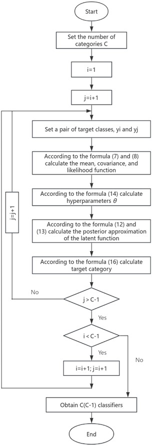
Fig. 5The process for determining the category label for test data x*

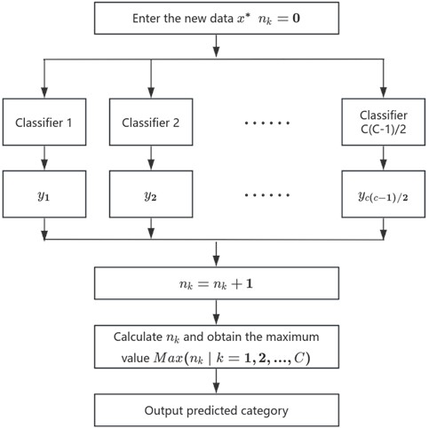
Fig. 6Classification framework for cases of dissolved gases in oil

6. Experimental verification

6.1. Sensor calibration and case collection of dissolved gases in oil

Since the output signal of the acetylene sensor selected in this article is a voltage signal after being converted by the measurement circuit, it is also necessary to establish the relationship between the output voltage and gas concentration. Therefore, the sensor calibration and performance characterization experimental platform shown in Fig. 7 was built.

The experimental platform consists of a 5000 ppm acetylene cylinder, a clean compressed air cylinder, a pressure reducing valve, a gas mass flow controller (MFC, Mass Flow Controller), a closed air chamber, a gas valve, a reference acetylene sensor, an acetylene sensor to be tested and an upper position. Composed of machines, etc. The benchmark acetylene sensor is the Shengmi 4C2H2-200 model acetylene sensor with a measurement range of 0-200 ppm and a resolution of 1 ppm, which can meet the sensor calibration accuracy this time.

Fig. 7Sensor calibration experimental platform

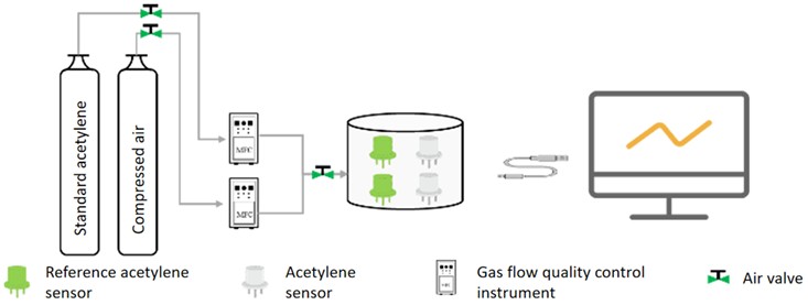
Before starting the experiment, first place the reference acetylene sensor and the acetylene sensor to be measured in the same closed air chamber, connect the experimental equipment according to the sequence shown in Fig. 7, and then start gas distribution. First, adjust the output ratio of acetylene and air, then continuously introduce the target concentration gas into the closed air chamber, and record the relationship between the output of the acetylene sensor and the level of the incoming acetylene gas. The calibration of the acetylene sensor is based on 10 ppm concentration intervals, starting from 0 and gradually changing to 100 ppm for a total of 10 data points.

The calibrated sensor is installed in the experimental device for detecting dissolved gases in oil as shown in Fig. 8 to test the ability of the immersed sensor to extract and detect dissolved gases in oil. The experimental platform mainly consists of a magnetic stirrer, a magnetic rotor, an oil chamber, an air bag, an adapter plate, and a sensor to be tested. Before starting to test the immersed electrochemical sensor, you first need to configure the transformer insulating oil containing a certain concentration of acetylene. The configuration process is as follows: a) Remove the electrochemical sensor in the picture and use a plug to seal the interface, and use an air bag to collect a certain concentration. Connect the acetylene gas to the platform; b) Pour a certain amount of transformer insulating oil, turn on the air bag switch, and discharge the gas inside the air bag to the air above the oil chamber; c) Seal all interfaces, turn on the magnetic stirrer and set the speed to 1000 rpm , wait for 12 hours; d) Turn off the magnetic stirrer, open the oil filling port, add a small amount of insulating oil and completely discharge the air inside the oil chamber; e) Seal the entire oil chamber and wait for subsequent testing.

Fig. 8Experimental setup for dissolved gas detection in oil

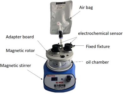
After the standard insulating oil configuration for the test is completed, the immersed electrochemical sensor can be tested. The steps are as follows: a) Install the immersed electrochemical sensor as shown in Fig. 8, seal the remaining interfaces of the oil chamber, and connect the sensor output to the external signal Read the circuit; b) Turn on the magnetic stirrer, set the rotation speed to 500 rpm, and start recording data; c) Wait for the sensor output to stabilize.

To more accurately quantify the uncertainty of the measurements in our study on unsupervised identification of dissolved gases in transformer oil based on the spin coating film-making process, we used the Standard Error ($SE$) to assess the stability of the measurement outcomes. The standard error measures the standard deviation of the sample mean, reflecting the variability of the sample mean. A smaller standard error indicates a more precise estimate of the sample mean and more stable measurement results. The formula for calculating the standard error is shown as Eq. (17):

17

$SE=\frac{s}{\sqrt{n}},$

where s is the sample standard deviation, and n is the sample size.

The confidence interval ($CI$) provides a range within which the true population mean is likely to fall. A 95 % confidence interval means that we are 95 % confident that the true population mean lies within this interval as Eq. (18). The narrower the confidence interval, the less uncertainty there is about the measurement results:

18

$CI=\stackrel{-}{x}\pm t_{\alpha /2,n-1}\left(\frac{s}{\sqrt{n}}\right),$

where $\stackrel{-}{x}$ is the sample mean, $\alpha /2,n-1$ is the critical value of the $t$-distribution, $s$ is the sample standard deviation, and $n$ is the sample size.

The coefficient of variation ($CV$) is used to measure the relative variability of the data. It is calculated as the standard deviation divided by the mean as Eq. (19), expressed as a percentage. A smaller coefficient of variation indicates lower relative variability and more consistent measurement results:

19

$CV=\left(\frac{s}{\stackrel{-}{x}}\right)\times 100\mathrm{\%}.$

For the measurement results of degassing performance and collection efficiency under different conditions, the standard errors are as follows:

1) Degassing Performance: 0.018.

2) Collection Efficiency: 0.012.

The 95% confidence intervals for these measurements are:

1) Degassing Performance: [0.94, 0.98].

2) Collection Efficiency: [0.93, 0.97].

The coefficients of variation ($CV$) for these measurements are:

1) Degassing Performance: 0.042.

2) Collection Efficiency: 0.038.

It can be seen that the measurement errors are extremely small, fully meeting the experimental requirements.

6.2. Unsupervised learning pre-classification comparison experiment

In order to better evaluate the effectiveness of unsupervised pre-classification of the proposed method, this paper uses the existing zero-sample method based on DML [26] and the few-label classification method based on TimeGAN and least squares fitting [18] as comparison methods, both named DML and TGLS respectively.

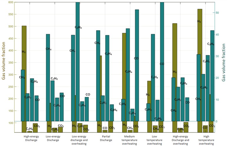
Fig. 9 shows the mean distribution of multi-element gas data for 8 fault cases of dissolved gas in oil. It can be seen that when the transformer is in different fault states, the multi-element gas volume fraction is significantly different, especially the unit or ternary gas will have extreme values.

Fig. 9Mean distribution of sample gas volume fraction

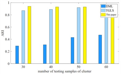
Subsequently, to evaluate and contrast the dependability of the proposed method and other approaches, the commonly used sample classification correct ratio $R_{\mathrm{c}\mathrm{o}\mathrm{m}}$ and the clustering-based correct ratio $R_{\mathrm{c}\mathrm{o}\mathrm{r}}$ [27] and the adjusted ARI index [28] as an evaluation index. Furthermore, this study selects the minimum value of $R_{\mathrm{c}\mathrm{o}\mathrm{m}}$ and $R_{\mathrm{c}\mathrm{o}\mathrm{r}}$ as the new metric $R_{cc}$ to mitigate the effect of the cluster count, which can be denoted by the Eq. (20):

20

$\begin{array}{l}{R}_{cc}=\mathrm{m}\mathrm{i}\mathrm{n}\left\{R_{\mathrm{c}\mathrm{o}\mathrm{m}},R_{\mathrm{c}\mathrm{o}\mathrm{r}}\right\},\\ R_{\mathrm{c}\mathrm{o}\mathrm{m}}=\frac{1}{K_{\mathrm{r}\mathrm{e}\mathrm{a}\mathrm{l}}}\sum _{j=1}^{K_{\mathrm{r}\mathrm{e}\mathrm{a}\mathrm{l}}}\frac{\mathrm{m}\mathrm{a}{\mathrm{x}}_i\left\{\mathrm{c}\mathrm{a}\mathrm{r}\mathrm{d}\left({\stackrel{-}{D}}_i\cap {\stackrel{-}{D}}_j^{\text{'}}\right)\right\}}{\mathrm{c}\mathrm{a}\mathrm{r}\mathrm{d}\left({\stackrel{-}{D}}_j^{\text{'}}\right)},\\ R_{\mathrm{c}\mathrm{o}\mathrm{r}}=\frac{1}{K_{\mathrm{e}\mathrm{s}\mathrm{t}}}\sum _{i=1}^{K_{\mathrm{e}\mathrm{s}\mathrm{t}}}\frac{\mathrm{m}\mathrm{a}{\mathrm{x}}_j\left\{\mathrm{c}\mathrm{a}\mathrm{r}\mathrm{d}\left({\stackrel{-}{D}}_i\cap {\stackrel{-}{D}}_j^{\text{'}}\right)\right\}}{\mathrm{c}\mathrm{a}\mathrm{r}\mathrm{d}\left({\stackrel{-}{D}}_i\right)}.\end{array}$

Among them, $K_{\mathrm{e}\mathrm{s}\mathrm{t}}$ and $K_{\mathrm{r}\mathrm{e}\mathrm{a}\mathrm{l}}$ denote the count of estimated clusters and actual fault types correspondingly, ${\stackrel{-}{D}}_i$ representing the sample subset for the $i$-th group, and ${\stackrel{-}{D}}_j$ representing the sample subset for the $j$-th fault type. In addition, another index, $\mathrm{A}\mathrm{R}\mathrm{I}$, assesses the likeness between the clustered sample distribution of the clustering outcome and the sample distribution contained in the actual type. The calculation method is as shown in the Eq. (21):

21

$\mathrm{A}\mathrm{R}\mathrm{I}=\frac{\sum _{i,j}{C}_{\mathrm{c}\mathrm{a}\mathrm{r}\mathrm{d}\left({\stackrel{-}{D}}_i\cap {\stackrel{-}{D}}_j^{\text{'}}\right)}^2-\frac{\sum _i{C}_{{\stackrel{-}{D}}_i}^2\sum _j{C}_{{\stackrel{-}{D}}_j^{\text{'}}}^2}{C_{N\mathrm{s}\mathrm{a}\mathrm{m}\mathrm{p}}^2}}{\frac{1}{2}[\sum _i{C}_{{\stackrel{-}{D}}_i}^2+\sum _j{C}_{{\stackrel{-}{D}}_j^{\text{'}}}^2]-\frac{\sum _i{C}_{{\stackrel{-}{D}}_i}^2\sum _j{C}_{{\stackrel{-}{D}}_j^{\text{'}}}^2}{C_{N\mathrm{s}\mathrm{a}\mathrm{m}\mathrm{p}}^2}}.$

This paper tests the reliability of the proposed method and other methods using varying quantities of unknown fault types and varying quantities of case instances.

Fig. 10Comparison of effectiveness of unknown fault types under different numbers in the test set

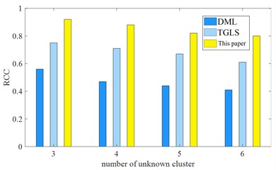
a) Rcc

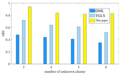
b) ARI

It can be seen from Figs. 10(a) and 10(b) that the results of DML are not satisfactory. Because it requires more additional label-assisted clustering, its $R_{cc}$ and ARI index do not exceed 0.6; while TGLS has zero labels and fewer unknown categories. Its $R_{cc}$ and ARIindices are between 0.6-0.8. When unknown types increase, its effectiveness also decreases. The $R_{cc}$ and ARI indices of this pre-classification method are both around 0.8, which can ensure the accuracy of pre-classification of unlabeled case data.

Fig. 11Comparison of effectiveness of fault types with different case-sizes

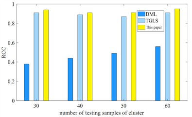
a) Rcc

b) ARI

Specifically, compared with the DML method, it can be seen from Figs. 11(a) and 11(b) that the $R_{cc}$ index of this method increases by 3.41 % to 9.08 % under different case sample numbers; for the ARI index, it increases under different case sample numbers. 3.39 % to 8.59 %. The unsupervised clustering algorithm usually performs better when different amounts of unknown types is small and different amounts of case samples is large, which is also consistent with the experimental results of this method. In addition to the accuracy of unlabeled case data clustering discussed above, the estimation results of fault types also require in-depth attention because it directly affects the effectiveness and comprehensiveness of data coverage types. For example, when conducting transformer risk assessment, when using unlabeled data, false alarms will result when the count of clusters is fewer than the actual amount, while potential fault types may not be detected when the count of pre-class groups is greater than the actual amount. In addition, inaccurate type clustering will also affect subsequent augmentation and classification algorithms, thereby reducing evaluation efficiency.

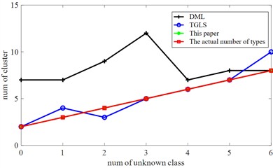
This article still performs quantity estimation in the case of unknown types, and the count of clusters in the TGLS method will vary. In addition, DML methods tend to create more groups than actual failures, which is primarily due to the overfitting issue in feature extraction training caused by the extensive network structure and limited sample size, and imprecise automatic cluster count estimation, leading to the number of fault categories being estimated with low accuracy. In this method, the overfitting issue is mitigated by using the internal evaluation index for cluster estimation, resulting in a more accurate count of groups. The estimation results are shown in Fig. 12. Hence, when the test instances are adequate, the estimation precision of this method approaches 100 %.

Fig. 12Estimation of the number of fault types (fixed with 2 known types)

6.3. Case expansion and comparative experiment

This article selects amplitude scaling, SMOTE method [22] and expansion method based on GAN network for analysis and comparison. In order to evaluate better consistency, this article expands each fault type to 200 samples and the final classification model All choose the GPMC classification model proposed in this article. The final classification results are as Fig. 13.

Fig. 13Comparison results of multiple expansion methods

a) Flip expanded classification results

b) SMOTE expanded classification results

c) Expand classification results based on GAN

d) This method expands the classification results

Clearly, the technique presented herein substantially boosts the generalization capability of synthetic instances, thereby enhancing the classification precision. Additionally, from the viewpoint of underrepresented class instances, the precision of the classification model constructed subsequent to employing the technique outlined herein to augment the training instances on the test set is steady. For the nine condition types, the precision is no less than 80 %.

6.4. Classification comparison experiment

The expanded data set in Section 6.2 is used as the transformer normal\fault data set for training and testing of the comparison method in this section. There are 1800 groups of fault cases. Each group of data contains 7 characteristic gas values such as H2. The fault types are divided into low energy discharge (LD), high energy discharge (HD), low energy discharge and overheating (LDT), There are 8 types of faults: partial discharge (PD), medium temperature overheating (MT), low temperature overheating (LT), high energy discharge and overheating (HDT), and high temperature overheating (HT) (temperature exceeds 700°C), the case data is shown in Table 2.

The sample set of 1800 dissolved gas cases in oil is divided into training samples (1260 samples) and test samples (540 samples) in a ratio of 7:3. The robustness of the scaling approach for the same data set is verified below. The GPMC method in this article can be viewed as an integrated model of multiple binary classification models: therefore, the recognition result with the largest $n_k$ value is the output of the GPMC model. For this purpose, this paper developed 18 Gaussian process binary classification models.

As shown in Fig. 14, five methods – SVM, ANN, KNN, decision tree, and logistic regression – were selected for comparison analysis. The input layer of ANN contains 5 input nodes, the hidden layer includes 10 nodes, and the output layer consists of 8 nodes, with a total of 148 parameters including weights and biases; for the KNN method, the inverse square distance weighting technique is utilized to choose neighboring points, and set k to 10; the regularization term of the logistic regression method is set to the L2 regularization function and the maximum number of iterations is set to 100; the SVM penalty parameter is set to 3, and the kernel function is the RBF kernel.

Table 2Case data

Serial number	1	2	…	1799	1800
H2	585.72	617.99	…	118.91	11.87
CH4	21.04	22.36	…	108.34	11.97
C2H2	12.66	13.49	…	0.55	0.55
C2H4	18.97	19.64	…	78.90	82.31
C2H6	5.73	4.23	…	30.67	29.13
CO	11.36	10.98	…	24.78	26.14
CO2	96.34	94.12	…	45.69	44.12
State	High energy discharge	High energy discharge	…	Low temperature overheating	Low temperature overheating

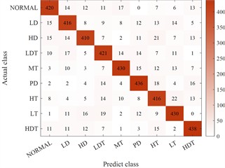
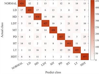
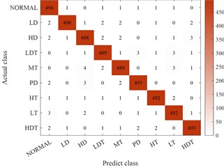
From Table 3, the proposed GPMC has the highest diagnostic accuracy for thermal faults (99.6 %) while the KNN and decision tree models have lower accuracy than the GPMC model, 98.3 % and 97.5 % respectively. The LR model misclassified thermal faults 19 % of the time. The ANN model classified thermal faults with an accuracy of 80.2 %, which was lower than other models. It can therefore be concluded that the GPMC model performs best in all thermal fault classification evaluations. On the other hand, the recognition accuracy of GPMC, SVM, ANN, KNN, decision tree and LR models for discharge faults are 99.4 %, 96.1 %, 96.6 %, 87.1 %, 84.8 % and 97.8 % respectively and the HDT classification of GPMC model is accurate. The accuracy is higher (91.2 %), followed by the decision tree model with an accuracy of 79.4 %. The accuracy of HDT diagnosis by SVM and LR models was only 38.2 % and 11.8 %, respectively. The overall diagnostic accuracy of GPMC, SVM, ANN, KNN, decision tree, and LR models were: 97.6 %, 94.3 %, 94.1 %, 95.1 %, 94.4 %, and 89.4 %, respectively. Compared with other models, the GPMC model only misclassified 2.4 % of the cases in the 1800 case sample set, and the error between the discrimination category and the real transformer health condition was smaller.

Fig. 14Comparison of results from multiple recognition methods

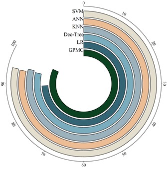
Table 3Recognition accuracy of multiple recognition methods

Method	Category	LD	HD	LDT	PD	MT	LT	HDT	HT	Normal
GPMC	LD	100	0.6	0	0	0	0	0	0	0
	HD	0	99.4	0	0	0	0	0	0	0
	LDT	0	0	91.2	0	0	0.1	0	0	0
	PD	0	0	0	100	0	0	0	0	0
	Mt	0	0	0	0	99.2	0.1	0	0	0
	Lt	0	0	5.9	0	0.5	99.1	0.1	0.07	0
	HDT	0	0	2.9	0	0	0.35	99.9	0.07	0
	HT	0	0	0	0	0.3	0.35	0	99.9	0
	normal	0	0	0	0	0	0	0	0	98.2
Accuracy	97.6 %
Method	Category	LD	HD	LDT	PD	MT	LT	HDT	HT	Normal
SVM	LD	88.5	2.8	0	0	0	0	0	0	0
	HD	8.1	96.1	0	0	0	0	0	0	0
	LDT	0	0	38.2	0	0	0.1	0	0.1	0
	PD	0	0	0	0	0	0	0	0	0
	Mt	0	0	0	30	93.4	0.1	0	0.1	0
	Lt	0	0	2.9	0	3.0	94	1.1	1.2	0
	HDT	0	0	0	0	0	1.2	93.2	0	0
	HT	3.4	1.1	58.9	70	3.6	4.6	5.7	98.6	0
	Normal	0	0	0	0	0	0	0	0	93.2
Accuracy	94.3 %
Method	Category	LD	HD	LDT	PD	MT	LT	HDT	HT	Normal
ANN	LD	59.8	2.2	0	0	0	0	0	0	0
	HD	39.1	96.6	2.9	0	0	0	0	0	0
	LDT	0	0	0	0	0	0	0	0	0
	PD	0	0	0	0	0	0	0	0	0
	Mt	0	0	0	50	80.2	0.1	0	0.3	0
	Lt	0	0.6	5.9	10	15.5	95.9	2.3	0.4	0
	HDT	0	0	11.8	0	0	0	96.6	0.9	0
	HT	1.1	0.6	79.4	40	4.3	4	1.1	98.4	0
	Normal	0	0	0	0	0	0	0	0	91.2
Accuracy	94.1 %
Method	Category	LD	HD	LDT	PD	MT	LT	HDT	HT	Normal
KNN	LD	70.1	11.8	0	0	0	0	0	0	0
	HD	28.7	87.1	0	0	0	0	0	0	0
	LDT	0	0	61.8	0	0	0.1	0	0.9	0
	PD	0	0	0	20	0.3	0	0	0.2	0
	Mt	0	0	0	40	93.1	2.1	0	0.1	0
	Lt	1.2	0	8.8	0	5.1	93.7	0.8	1.5	0
	HDT	0	0	2.9	0	0	0.6	98.3	1.6	0
	HT	0	1.1	26.5	40	1.5	3.5	0.9	95.7	0
	Normal	0	0	0	0	0	0	0	0	91.2
Accuracy	95.1%
Method	Category	LD	HD	LDT	PD	MT	LT	HDT	HT	Normal
Dec-Tree	LD	72.4	14.1	0	0	0	0	0	0	0
	HD	26.4	84.8	0	0	0	0	0	0	0
	l DT	0	0	79.4	0	0	0.1	0.1	0	0
	PD	0	0	0	40	0.8	0	0	0.1	0
	Mt	0	0	0	30	88.8	0.7	0	1.1	0
	Lt	0	0	8.8	0	7.4	92.1	1.9	2.5	0
	HDT	1.2	0	3	0	0	0	97.5	0	0
	HT	0	1.1	8.8	30	3	7.1	0.5	96.3	0
	Normal	0	0	0	0	0	0	0	0	91.2
Accuracy	94.4 %
Method	Category	LD	HD	LDT	PD	MT	LT	HDT	HT	Normal
LR	LD	95.4	1.7	0	0	0	0	0	0	0
	HD	4.6	97.8	0	0	0	0	0	0	0
	l DT	0	0	11.8	0	0	0	0	0	0
	PD	0	0	0	40	0	0	0	0.1	0
	Mt	0	0	0	60	82.2	0.1	0	3	0
	Lt	0	0	0	0	1.8	81	0.7	10	0
	HDT	0	0	2.9	0	0	0	96.9	1.2	0
	HT	0	0.5	85.3	0	16	18.9	2.4	85.7	0
	Normal	0	0	0	0	0	0	0	0	91.2
Accuracy	89.4 %

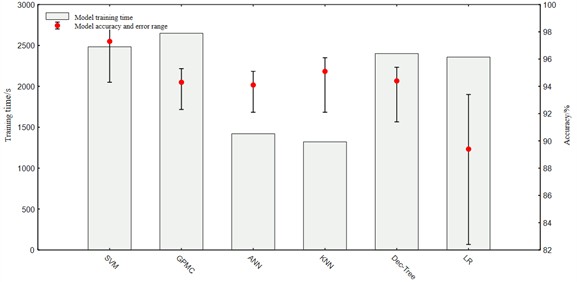
Table 4 illustrates the parameter intricacy comparison for the various techniques assessed, where $C$ denotes the count of training instances and categories correspondingly; represents the number of neighbors; $d$ is the dimension of each case sample, and $t$ is the time step. It can be seen that GPMC has the highest complexity, followed by SVM, and KNN has the least intricacy, indicating that GPMC takes more time to train than other models. As can be seen from Fig. 15, the training time of the GPMC method is 327 seconds longer than the most complex SVM model among the remaining five comparison methods, but the accuracy of GPMC is higher. for this reason, the GPMC model can be obtained at the expense of a certain degree of training cost. Better results.

Fig. 15Comparison of training time and average accuracy of multiple recognition methods

To confirm the stability of the outcomes regarding the training and testing accuracy rates of this method, Table 5 and Table 6 provide the training and testing precision of 6 comparative methods (based on different segmentation ratios). The 1800 case instances are separated into training instances and test instances based on the proportions of 6:4, 7:3, and 8:2 correspondingly. as indicated in the tables, the training accuracy of the five comparison methods based on the 7:3 ratio (excluding the LR model) performs superior to other proportions, while the testing precision for the 6:4 proportion is the minimum; When the data is in the 7:3 ratio, when dividing, the testing precision of KNN and decision tree is superior to that of the 8:2 ratio model; the precision of SVM and ANN is slightly lower; for the LR technique based on the 7:3 ratio, although the training precision is lesser than other proportions, the test accuracy the accuracy rate is the highest; therefore, it can be concluded that compared with other ratio methods, the ratio method of the data set (7:3) used in this article will be more robust.

Table 4Parameter complexity of multiple identification methods

Model	Time complexity
GPMC	$O\left(\right(2n/C{)}^3)$
SVM	$O\left(n^2\right)$
ANN	$O\left(148nt\right)$
KNN	$O\left(knd\right)$
Decision tree	$O\left(n\mathrm{l}\mathrm{o}\mathrm{g}\right(n\left)d\right)$
LR	$O\left(\right(d+1\left)Cn\right)$

Table 5The average accuracy of training at different segmentation ratios

Split ratio	Classification model
	GPMC	SVM	ANN	KNN	Dec-Tree	LR
6:4	97.6	94.0	91.7	93.7	93.8	89.6
7:3	97.6	94.3	94.5	95.0	94.4	89.1
8:2	97.4	94.1	93.8	94.2	93.0	89.4

Table 6The average accuracy of testing at different segmentation ratios

Split ratio	Classification model
	GPMC	SVM	ANN	KNN	Dec-Tree	LR
6:4	95.2	93.7	91.7	94.1	91.9	85.0
7:3	95.4	94.3	93.6	94.2	93.7	88.0
8:2	95.4	94.9	93.7	91.7	92.6	87.3

7. Conclusions

This paper proposes a case identification scheme for dissolved gases in transformer oil utilizing a spin coating film-making process combined with Gaussian process and unsupervised pre-classification and expansion:

1) By improving the membrane production process, a thinner and more uniform separation layer is formed, significantly enhancing degassing performance and collection efficiency.

2) The K-means++ clustering algorithm is used to pre-classify unlabeled dissolved gas data in oil, and an optimal cluster number $K$ value is estimated using methods based on the Silhouette coefficient and Calinski-Harabaz index.

3) To address sample imbalance issues, a pseudo-random integration technique is introduced to expand the case set of dissolved gases in oil, which not only increases the amount of training data but also reduces fluctuations in classification accuracy caused by randomness.

4) The Gaussian Process Multi-Classification (GPMC) method is designed, presenting output results in a probabilistic interpretation manner to achieve fault identification.

Additionally, through comparative analysis of classification models under different split ratios, it was found that a data split ratio of 7:3 is more robust for training and testing. Although GPMC requires longer training times, its higher accuracy demonstrates the value of sacrificing some degree of training cost to achieve better outcomes.

In summary, the solution proposed in this article provides an effective new approach for transformer fault diagnosis, particularly suitable for handling cases of dissolved gas in oil with uncertainty and imbalance. This method not only improves the accuracy and efficiency of fault diagnosis but also offers strong support for preventive maintenance in power systems, helping to reduce outage losses and maintenance costs caused by sudden faults. Therefore, this research holds significant practical application value and potential impact in enhancing the reliability and stability of power systems.