Abstract
Electrocardiogram (ECG) signals often encounter various types of noise interference, which annihilates their waveform characteristics and exhibits strong instability. To facilitate clinical diagnosis and analysis, it is necessary to perform denoising processing in advance. A denoising method for ECG signals based on variational mode decomposition (VMD) and recursive least square (RLS) has been proposed. VMD was used for the modal decomposition of noisy ECG signals, and the recursive least square (RLS) algorithm was used for adaptive filtering of various intrinsic mode functions (IMFs) components. The problem construction, solution, and decomposition characteristics of VMD were analyzed. The IMFs filtered by RLS were reconstructed. This achieved the elimination of interference noise in the ECG signal. The Sym8 wavelet basis, LMS, NLMS, RLS, and VMD-RLS denoising method were compared by using ECG signals including Gaussian white noise, baseband drift, electrode motion, electromyographic interference, and electrical interference noise. The experimental results showed that the VMD-RLS denoising method has significantly better denoising performance than the other four methods, achieving better values in the quantitative evaluation indicators. This algorithm improved convergence speed and signal estimation accuracy, and it has good effectiveness, superiority, and practicality. Therefore, the VMD-RLS denoising method can enable doctors and researchers to analyze and diagnose ECG signals of heart diseases more accurately.
Highlights
- A denoising method based on variational mode decomposition (VMD) and recursive least square (RLS) is proposed for ECG signals.
- The proposed algorithm is compared with the Sym8 wavelet basis, LMS, NLMS, and RLS.
- The ECG signals including Gaussian white noise, baseband drift, electrode motion, electromyographic interference, and electrical interference noise are respectively used to verify proposed method.
- The proposed method has significantly better denoising performance than the other four methods, and has good effectiveness, superiority, and practicality.
1. Introduction
Electrocardiogram (ECG) is an electrical signal used to capture the heartbeat. [1-3]. The cells surrounding the heart carry associated charges that cause the heart to depolarize with each heartbeat. This process will present small electrical signals on the surface of the skin, which can be collected and displayed for analysis on an electrocardiograph.
ECG is a quasi-periodic time series signal that exhibits nonlinear and non-stationary characteristics. It represents the flow of ionic currents that lead to the contraction and relaxation of cardiac fibers, indirectly reflecting myocardial activity. It is a time-varying bioelectric signal that has been widely used to check cardiac vitality and myocardial function [4-6].
ECG signals have two different types of features, one of which is morphological features: P wave, T wave, U wave, and QRS complex. Another type of interval feature is: PR segment, ST segment, PR interval, RR interval, ST interval, etc. ECG is widely used in clinical diagnosis, such as cardiopulmonary monitoring, biometric authentication, ECG rhythm, and heart rate variability assessment [7].
Accurate analysis of these features depends on correctly identifying the characteristics of the recorded ECG signal morphology and intervals. However, ECG signals are susceptible to various main noises, which greatly affect the analysis and processing of ECG signals [8]. This may distort the morphological and interval characteristics of ECG leads, leading to misdiagnosis and inappropriate treatment for patients.
In order to extract correct physiological information, it is essential to eliminate the noise present in the ECG signal [9]. ECG signal denoising is a critical area of research that focuses on removing this noise, enabling doctors and researchers to analyze and diagnose heart diseases more accurately.
Currently, significant progress has been made in research on ECG signal denoising. Many scholars have proposed various filter methods, including wavelet transform, singular spectrum analysis, sparse representation, deep learning, multimodal signal processing, and adaptive filtering for ECG signal denoising [1, 10-11].
Among these, the filter is the most commonly used method for denoising ECG signals. The types of filters typically employed include low-pass filters, high-pass filters, and band-stop filters. These filters can filter out noise signals in different frequency ranges [12]. However, appropriate filters should be selected based on the specific application scenario. When selecting a filter, one should consider factors such as the frequency range of the signal, the characteristics of the noise, and the specific parameters of the filter.
Various wavelet transforms methods have also been used for signal filtering processing, improving the signal-to-noise ratio, with significantly better results than filter methods [13-14]. It eliminates noise by decomposing the ECG signal into wavelet coefficients of different frequencies, and then processing the wavelet coefficients. The wavelet transform method has good time-frequency localization characteristics, which can better preserve the local features of ECG signals. However, wavelet functions do not have uniqueness and can often only be selected and parameters determined through continuous experimentation [15-16].
Singular spectrum analysis is a method based on the frequency domain representation of signals, which can identify the noise components in ECG signals and perform corresponding elimination [17]. This method can better preserve the dynamic characteristics of ECG signals. However, it is quite sensitive to non-Gaussian noise, which limits the application of singular spectrum analysis methods in containing outliers.
Adaptive filtering is a widely used method for denoising ECG signals. This method involves adjusting filter parameters based on the characteristics of the signal itself to effectively reduce noise. It is designed to adapt to complex signal environments and performs well with nonlinear signals. Common adaptive filtering methods include adaptive mean filter, adaptive median filter, adaptive linear combination filter, least mean square (LMS), normalized least mean square (NLMS), and RLS [18-20]. Linear adaptive filters and corresponding algorithms are widely used due to their advantages of simple structure and low computational complexity. Among these, the RLS algorithm is a type of fast algorithm of the least squares algorithm, which overcomes the drawbacks of LMS algorithm, such as slow convergence speed and poor adaptation to signal non-stationarity, by using the square error and minimum criterion for re-estimation of all input signals at each moment.
Recently, various emerging denoising methods have gained popularity in the field of ECG signal processing, including sparse representation and deep learning methods [21-23]. Sparse representation is a method of reducing signal noise by finding the sparsest representation. Researchers have utilized sparse representation methods for ECG signal denoising by selecting the most appropriate atoms to accurately represent the signal, effectively suppressing noise in the process. However, this approach requires selecting appropriate basis vectors and adjusting parameters for different datasets. Additionally, error accumulation may occur when processing noisy data, which affects the accuracy of the algorithm. On the other hand, deep learning has demonstrated significant potential for ECG signal denoising. Researchers deploy deep neural networks to remove noise from ECG signals. By leveraging large amounts of training data and complex network architectures, it is possible to effectively eliminate noise while preserving essential features of the ECG signals. Nevertheless, this method demands substantial amounts of training data and computational resources.
Researchers have also utilized multimodal signal processing methods to complement multimodal signals and design more effective denoising algorithms, thereby improving the quality of ECG signals. Dragomiretskiy recently proposed a multimodal component signal adaptive decomposition method in 2014, namely variational modal decomposition [24]. The decomposition process of this method is to iteratively search for the optimal solution of the variational model to determine the frequency center and bandwidth of each component, thereby adaptively achieving frequency domain decomposition of the signal and effective separation of each component. Compared to empirical mode decomposition (EMD), VMD functions similarly to a set of adaptive Wiener filters. Unlike EMD methods, VMD does not suffer from inherent modal aliasing, demonstrating improved noise robustness.
Considering the above analysis, a VMD-RLS joint filtering algorithm is proposed to eliminate the effects of noise in weak ECG signals, which are often affected by various interference sources. This algorithm leverages the strengths of both VMD and RLS algorithms. The process begins by decomposing the noisy ECG signal into multiple band-limited intrinsic mode functions (IMFs) using the VMD algorithm. Next, each IMF component is filtered using the RLS algorithm. Finally, the “clean” data and the filtered IMFs are reconstructed to produce a denoised signal, effectively completing the denoising process.
2. Denoising method
2.1. Variational mode decomposition
The essence of VMD algorithm is to decompose the electrocardiogram signal to be analyzed into a series of sparse intrinsic mode functions (IMFs) by solving the constructed constrained variational problem. This process seeks to minimize the sum of bandwidths of each modality while constraining the sum of all modalities to be consistent with the original signal. The specific steps for constructing and solving variational problems are as follows [24-27].
(1) Assuming that original signal is a multi-component signal, consisting of (predetermined scale) finite bandwidth intrinsic mode function components , as shown in Eq. (1), and its center frequency is :
where, is instantaneous amplitude, and is instantaneous frequency.
(2) Determine the number of , and then use Hilbert transform to calculate the relevant analytical signals, and then obtain the single-sided spectrum, and divide the width of the signal frequency band:
where, is the Dirichlet function.
(3) Mix the frequencies of each with the exponential signal of the corresponding center frequency to achieve the spectral shift of the sub signals. Transfer spectrum for to corresponding baseband:
(4) Based on the Gaussian smoothness and gradient squared -norm criteria of demodulated signal mentioned above, each mode bandwidth can be estimated, and the constrained VMD variational model can be represented as:
where , , .
(5) To find optimal solution of the constrained variational model in step (4), it must be transformed into an unconstrained variational problem. A quadratic penalty factor is introduced to ensure convergence even in the presence of Gaussian noise. Additionally, the Lagrangian multiplication operator is introduced to maintain strict constraint conditions. Construct an augmented Lagrangian expression as shown in Eq. (5):
(6) Using alternating direction multiplier method (ADMM) to solve Eq. (5), combined with Fourier Isometric Transform, , , and are transformed into the frequency domain for alternating iteration, optimizing to obtain the corresponding modal components and center frequency, and searching for the saddle point of the augmented Lagrangian expression. The convergence condition for iteration number is:
The optimal iterative solution obtained is:
Once the convergence accuracy is met or the maximum number of iterations is reached, the iterations are stopped. In this case, the original signal can be decomposed into mode components :
Therefore, by constructing and solving the variational modal problem, VMD algorithm can be realized as follows:
(1) Initialize , , , .
(2) .
(3) Update A and B using Eqs. (5) and (6).
(4) Update the step size according to Eq. (8), and set as noise tolerance parameter. When the signal noise is serious, to get a better denoising effect, can be set:
(5) If the convergence accuracy is met, stop iterations and output , otherwise go to step (2) to continue.
The choice of appropriate and has a large impact on the effectiveness of the decomposition of the VMD algorithm. If is too small, there will be aliasing between modal components. If is too large, it will cause modal over decomposition, and the same frequency component will be decomposed into multiple modalities, resulting in false components. And determines the bandwidth of each modality. The smaller is, the larger the bandwidth of each IMF component is. Conversely, the smaller the bandwidth of component, even, too large can lead to the loss of important information.
Considering the interaction between parameters and , if one parameter is fixed separately and the other parameter is optimized, the results obtained are only relatively optimal. Therefore, it is necessary to optimize both parameters simultaneously. GWO algorithm is a newly proposed swarm intelligence optimization algorithm in recent years, which has good global optimization ability [28]. Here, the GWO algorithm is used to perform parallel optimization on two decomposition parameters, automatically selecting the best parameter combination.
2.2. Recursive least square
The least squares algorithm is another widely used classic algorithm in adaptive algorithms. Recursive least squares algorithm (RLS) is an upgraded algorithm based on the least squares algorithm, and its theoretical foundation is also the steepest descent algorithm. The cost function of the RLS is different from that of the LMS. The algorithm uses an exponential weighting method to describe the cost function, and its objective function expression is as follows [19, 29-31]:
where, is the expected output of the observed signal, is the actual output of the observed signal, is the observed input signal, and is the filter tap coefficient. represents the forgetting factor, with a range of [0, 1), which assigns weights to all samples. The closer the sample is to the current moment, the greater its contribution to the objective function.
Calculate the autocorrelation matrix of the input signal to obtain:
Calculate the cross-correlation vector between and :
The Eqs. (12) and (13) satisfy the following recursive relationships, respectively:
Calculate the inverse matrix of and obtain:
Among them, the expression of in Eq. (16) is:
The Eq. (17) represents the Kalman gain vector at that time. By using Eqs. (12) and (13) to calculate the autocorrelation matrix and cross correlation vector, the optimal solution for the filter tap coefficients can be iteratively obtained.
Therefore, the basic principle of the RLS is to calculate the latest estimation of the -th iteration weight vector based on the newly obtained data, given the least squares estimation of the 1-th iteration filter tap weight vector. The purpose of its algorithm is to select the coefficients of adaptive filtering, so that the output signal during observation matches the expected signal in the least squares sense.
The steps of the RLS are as follows:
(1) At moment , set the forgetting factor , set the filter tap coefficient , and the inverse matrix of the autocorrelation matrix:
where, is a normal number and can be used as the power estimation of the tap input signal.
(2) Calculate the instantaneous error at time :
(3) Calculate the Kalman gain vector at time :
(4) Calculate the inverse matrix of the autocorrelation matrix:
(5) Update the tap coefficients of the adaptive filter:
(6) Make .
(7) Repeat steps (2) to (6) until the iteration process is completed.
The RLS adaptive filtering algorithm is a special case of the Kalman filtering algorithm and belongs to the recursive algorithm of the adaptive lateral filtering algorithm. Due to the application of matrix inversion in the derivation process of the algorithm, the RLS can achieve fast convergence. Moreover, the diffusion of the eigenvalues of the input signal correlation matrix (the ratio of maximum to minimum eigenvalues) is relatively robust, thus breaking through many shortcomings and limitations of the LMS. The convergence speed is one order of magnitude faster than the general LMS, and the convergence rate of the RLS algorithm does not change with the diffusion degree (i.e. the condition number) of the eigenvalues of the autocorrelation matrix of the input vector .
The reason is that the RLS filtering algorithm whitens the input data (assuming the mean is zero) by utilizing the inverse of autocorrelation matrix of input data, resulting in improved performance, but the cost is an increase in the computational complexity of the algorithm. As the number of iterations approaches infinity, the excess mean square error of the algorithm converges to zero.
2.3. Denoising methods based on VMD and RLS
ECG signal is a kind of nonlinear, non-stationary, random, and quasi-periodic weak physiological signal. ECG signals are easily disturbed by instruments, human activities, operators, and the surrounding environment. VMD algorithm can decompose ECG signals completely, but sometimes it can't highlight weak P wave, Q wave, S wave, and T wave. Because of the good adaptability of RLS algorithm to non-stationary signals, and its advantages such as fast convergence, high estimation accuracy, and good stability, adaptive filtering can eliminate most of the noise in ECG signals. To keep the useful characteristic information of ECG signal while eliminating the noise of ECG signal, an ECG signal denoising method based on VMD and RLS is proposed.
From Eqs. (9) and (11), it can be concluded that:
where, the was used to adjust the proportion of each IMF. The optimal coefficient for minimizing can be obtained by differentiating Eq. (24) with respect to and setting the derivatives to zero. This yields the following equation:
Then it can be obtained:
By defining:
Then Eq. (26) can be expressed as:
Considering all the values of the index and , the following matrix can be obtained:
This also can be denoted as:
And the optimal coefficients can be obtained:
To compute the will result in an algorithm with computational complexity of . Here computes the by means of the Matrix Inversion Lemma:
where:
A prior error can be defined as:
By expressing as a function of a prior error and can be expressed as:
From the mathematical argument, is the estimated value of the true response ECG signal. can enable the RLS algorithm to track non-stationary signals normally. The larger the forgetting factor , the slower the convergence speed of the RLS algorithm, but the smaller the noise after the weight coefficients converge. For weak ECG signals, can choose to be close to 1. The key element of using VMD-RLS is to enhance the estimation of global interference by applying a linear relationship between the decomposed IMFs and the long-distance measurements.
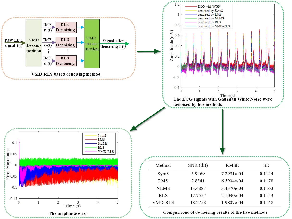
The implementation of this method is to first decompose the ECG signal into a set of modal components using VMD, and then RLS adaptive denoising is performed on each modal component separately. Finally, the denoised ECG signal is reconstructed by combining the results obtained from RLS denoising. The process of this denoising method is shown in Fig. 1.
Fig. 1The structure diagram of VMD-RLS based denoising method
2.4. Performance evaluation
To evaluate the performance of the denoising algorithm in this article, the signal-to-noise ratio (SNR), root mean square error (RMSE), and standard deviation (SD) between the filtered signal and the original signal were compared [31]. If represents a clean ECG signal and represents an estimated ECG signal after network denoising, SNR is defined as the ratio of the signal to noise, and in decibels (dB). As an important indicator for evaluating signal quality, a higher SNR value indicates better filtering performance. The expression is shown in Eq. (37):
RMSE is a dimensionless parameter, which represents the difference between the filtered estimated signal and the real signal. The lower its value, the better the filtering performance. The expression is shown in Eq. (38):
The SD is the square root of the average of the squared deviations between each estimate and its mean. In a statistical sample, the larger the SD, the more dispersed the distribution of its estimated values, and the worse its central tendency. On the contrary, the smaller the SD, the more concentrated the distribution of its estimated values, and the better its central tendency. The expression is shown in Eq. (39):
3. Experiment and analysis
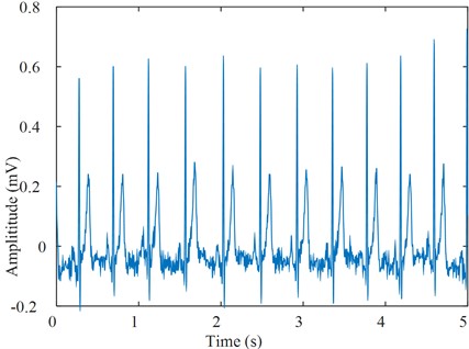
ECG is recorded by capturing the potential difference between two electrodes. However, in experimental acquisition, ECG signals are susceptible to various major noises. The main noise of its ECG signal includes Gaussian white noise, baseband drift, electromyographic interference, power frequency noise, and other noise interferences. For this reason, the ECG signal denoising here mainly focuses on these situations through experiments and analysis. The dataset is from Physionet ECG Database, and the noise free ECG signal is obtained as shown in Fig. 2.
3.1. Gaussian white noise
During the process of collecting ECG signals, white noise interference is often encountered. Gaussian noise is used here to better simulate the unknown real noise during the electrocardiogram acquisition process. In practical applications, noise amplitude is random at any time, but it satisfies Gaussian distribution.
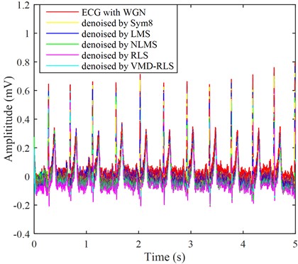
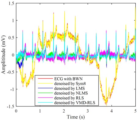
The used signal is a noise-free signal from the Physionet ECG Database signal database, as shown by adding Gaussian white noise as interference noise to the ECG signal in Fig. 2, as shown by the red line in Fig. 3. It can be seen from the Fig. 2 that the red line has the highest ECG amplitude, and in the weak P wave, Q wave, S wave, and T wave areas, almost all are submerged by white noise, unable to highlight the ECG characteristic signal, which is not conducive to clinical diagnosis.
Fig. 2The ECG signal without noise
The VMD-RLS mentioned in the article was used for denoising, and the denoised ECG signal is shown in the blue line by Fig. 3. In weak P wave, Q wave, S wave, and T wave regions, the noise was significantly reduced, and the ECG morphological features were highlighted.
In order to compare with other denoising methods, Sym8 wavelet basis, LMS algorithm, NLMS algorithm, and RLS direct denoising were used to obtain the denoised signals as shown by yellow, blue, green, and purple in Fig. 3.
The signals after denoising using five methods were analyzed and compared with the ECG signals and noisy ECG signals in the original Fig. 2. In Fig. 3, it can be clearly seen that the blue ECG signal denoised by VMD-RLS has the best denoising effect, especially in the weak P wave, Q wave, S wave, and T wave regions, where the white noise amplitude is almost eliminated. The yellow and blue ECG signals after Sym8 wavelet basis and LMS denoising are not significantly denoised, and they are almost identical to the red signal without denoising treatment. The signal denoised by NLMS shows no significant noise reduction in the first 1s period, while the remaining period shows good noise reduction. The amplitude of the purple ECG signal directly denoised by RLS is slightly larger than that of the signal denoised by VMD-RLS, but the entire signal range maintains good consistency.
To further demonstrate the denoising effect of VMD-RLS, Fig. 4 shows a comparison of the amplitude error between the original signal and the denoised ECG signals by Sym8, LMS, NLMS, RLS, and VMD-RLS algorithms. In Fig. 4, it can be seen that the amplitude error of the VMD-RLS algorithm after denoising is smaller than that of the Sym8, RLS, LMS, and NLMS algorithms. The experimental results showed that the convergence performance of the Sym8, LMS, and NLMS algorithms deteriorates due to the influence of large noise. Compared to Sym8, RLS, LMS, and NLMS algorithms, VMD-RLS algorithm has better convergence performance and can better approximate the expected signal.
In order to quantitatively evaluate the five types of denoising effects, the SNR, RMSE, and SD are used as performance evaluation indicators for denoising. Thus, quantitatively expressing the difference in filtering and denoising effects on ECG signals containing Gaussian white noise. After the denoising experiment, the denoising performance evaluation indicators of the five methods are shown in Table 1.
Fig. 3The ECG signals with Gaussian white noise were denoised by four methods
In Table 1, it shows that the SNR after VMD-RLS denoising is the highest and the RMSE is the smallest, indicating the best effect. The SD is close to the minimum, indicating that the more concentrated the distribution of signal values after denoising, the better the central tendency. The SNR and RMSE values after direct RLS denoising are slightly smaller than the former, indicating that the denoising effect and the concentration of signal value distribution after denoising are not as good as the former. In addition, the noisy ECG signal is fully decomposed into multiple band limited modal function signals through VMD, and even if the signal is sparsified, it is beneficial for further denoising the noisy signal. The SNR and SD of the signal denoised by Sym8 are the smallest, and the RMSE is the largest, indicating that although the signal value distribution is most concentrated after denoising, the denoising effect is the worst. The SNR and RMSE after LMS denoising are close to Sym8, with the largest SD, indicating that the denoising effect is close to the worst compared to Sym8, and the signal value distribution after denoising becomes more dispersed, with the worst central tendency. The SNR after denoising using the NLMS method is twice that of LMS, but less than that of RLS. The RMSE value is only half of LMS, indicating that the denoising effect is twice better than LMS. Similarly, the RMSE value is also between the two, indicating that the denoising effect is between the two. In addition, after multiple experiments, the five denoising methods may vary in the denoising analysis results for different simulated signals, but the effect is still best based on the VMD-RLS denoising method.
Fig. 4The amplitude error
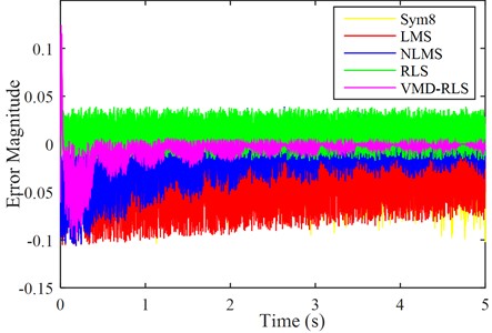
Table 1Comparisons of de-noising results of the five methods
Method | SNR (dB) | RMSE | SD |
Sym8 | 6.9469 | 7.2991e-04 | 0.1144 |
LMS | 7.8341 | 6.5904e-04 | 0.1178 |
NLMS | 13.4887 | 3.4370e-04 | 0.1163 |
RLS | 17.7557 | 2.1030e-04 | 0.1153 |
VMD-RLS | 18.2758 | 1.9807e-04 | 0.1148 |
3.2. Baseline Wander noise
Baseline drift is a type of low-frequency signal artifact. It is the instantaneous baseline drift caused by the impedance between the electrode and skin as the electrode moves. The amplitude of baseline drift can sometimes exceed several times that of the QRS complex. The amplitude and duration of motion artifacts generated in this way can reach 500 % of the ECG peak and 300-500 ms. It has the greatest impact on ECG signals and exhibits significant amplitude jitter. Therefore, ECG signals disturbed by such noise exhibit distortion and jitter, making it difficult to accurately locate the location of ECG feature points.
Severe baseline drift will distort the ST segments and low frequencies of the ECG, leading to misdiagnosis of Brugada syndrome, myocardial infarction, and other ST segment abnormalities. In order to obtain effective ECG signals, such noise must be eliminated.
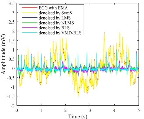
By adding low-frequency signals as interference noise to the ECG signal in Fig. 2, as shown by the red line in Fig. 5. From the graph, we can see that the ECG amplitude of the red line fluctuates significantly, and the presence of baseline drift has already affected the overall waveform trend, resulting in a clear upward and downward trend of the original ECG signal. Part of the signals have already exhibited ECG characteristic signals, and as can be seen from the local detail maps of noisy signals, baseline drift causes normal ST-segment elevation to become convex upward, which is not conducive to clinical diagnosis. Using the same method, the ECG signal with baseline drift was denoised using the VMD-RLS denoising method, RLS denoising method, LMS denoising method, NLMS denoising method, and Sym8 denoising method. The resulting waveforms are shown in the ECG with blue, purple, blue, green, and yellow lines in Fig. 5, respectively.
Fig. 5The ECG signals with baseline wander noise were denoised by four methods
In Fig. 5, it can be seen that the blue-green ECG signal denoised based on VMD-RLS is compared with original ECG signal in Fig. 2. It shows that the denoised signal returns to the baseline, and its morphology remains basically consistent with the original signal. Especially from the local details of the denoised ECG signal, it can be observed that the ST segment of the ECG signal has returned to its normal waveform.
Although the ECG signal after noise reduction using RLS denoising method, LMS denoising method, and NLMS denoising method has basically returned to the baseline, and the original signal remains basically consistent. However, during the first 0.5 seconds, there was still some baseline drift that was not completely eliminated. Moreover, the ECG signals after noise elimination by the LMS noise cancellation method and the NLMS noise cancellation method leave more baseline drift. The effect after Sym8 denoising is the worst, with almost no change.
3.3. Electrode movement noise
Electrode contact noise is caused by poor contact between the electrode and the skin or electrode detachment, resulting in occasional absence of electrocardiogram recording and rapid step changes in the electrocardiogram. If this interference persists for a longer period of time or greater magnitude, it is necessary to promptly issue a warning to the user and relocate the body surface collection electrode.
Motion interference is a sudden change signal. Its generation is due to the relative displacement of the contact point between the electrode and skin caused by human movement, resulting in impedance changes and potential changes; The second reason is that during the electrocardiogram collection process, the movement of other objects in the surrounding environment causes changes in the potential on the electrode. The fluctuation of motion interference is large and belongs to an irregular waveform form, so motion interference will completely annihilate the waveform features, thereby losing electrocardiogram information. During the collection process, the tested person is in a constantly changing motion environment, so the influence of motion interference on the electrocardiogram signal is very common, and its spectrum overlaps with the electrocardiogram signal in a large area.
Fig. 6The ECG signals with electrode movement noise were denoised by four methods
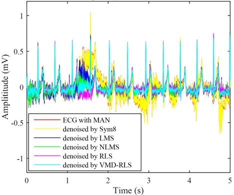
By adding electrode motion noise to the ECG signal in Fig. 2, the results are shown in the red line in Fig. 6. The baseline of ECG signal with the red line undergoes continuous changes, changing the morphology of the characteristic waves in the original ECG signal, which has seriously led to the unreadable ECG signal. It is necessary to evaluate the quality of this electrocardiogram signal, and then exclude the severely disturbed noise from the analysis range to reduce misjudgment. Using the same method, the ECG signal with electrode motion interference was denoised using VMD-RLS denoising method, RLS denoising method, LMS denoising method, NLMS denoising method, and Sym8 denoising method. The resulting waveforms are shown in the ECG with blue, purple, blue, green, and yellow lines in Fig. 6, respectively.
The blue-green ECG signal denoised based on the VMD-RLS is compared with original ECG signal in Fig. 2. The denoised ECG signal returns to the baseline, and its morphology is basically consistent with the original signal. Especially from the local details of the denoised ECG signal, it can be found that the ECG signal has returned to normal waveform in weak P-wave, Q-wave, S-wave, and T-wave areas.
After the RLS denoising method, LMS denoising method, and NLMS denoising method were used to eliminate noise, the ECG signal returned to the baseline and the original signal remained consistent. However, during the first 0.5 seconds, there were still some motion artifacts that were not completely eliminated. During the first 0.5 seconds, the RLS denoising method achieved almost the same effect as VMD-RLS denoising, but the local noise amplitude was still larger throughout the entire signal period than the latter. From the figure, it can be seen that similarly, the ECG signal that has been denoised using LMS and NLMS methods still has a significant amount of local noise remaining in the negative direction of the signal. Like baseline drift denoising, the effect of Sym8 denoising is the worst, with almost no change.
3.4. Muscle artifacts noise
Each person’s skin surface has an electric potential of about 30 mV. This data is generally maintained between 25-35 mV, and 5 mV interference is sufficient to affect ECG signals. Due to the trembling of muscle fibers, changes in surface potential can occur, which affects the potential difference collected by electrode patches on the surface and causes electromyographic interference. This generally lasts for a short period, causing small ripples in the ECG signal waveform. The frequency distribution range of this noise is relatively wide, generally between zero and 10000 Hz, but relatively more are distributed between 30-300 Hz, with frequency characteristics equivalent to white noise. This interference is caused by the electrical activity of muscles during contraction or sudden bodily movements which is also known as muscle artifact (MA).
The MA can cause local waveform distortion of ECG signals. This makes it very challenging to denoise ECG signals to accurately identify various ECG arrhythmias. Due to its wide frequency distribution range, traditional denoising methods have not achieved ideal results. This is because general denoising methods can only effectively remove distributed noise in specific frequency bands, so electromyographic interference has always been a research difficulty.
To verify the VMD-RLS denoising method proposed in this article, muscle artifact noise was added to the ECG signal in Fig. 2, and the results are shown in the red line in Fig. 7. From the graph, the ECG signal with the red line undergoes continuous and irregular rapid changes in the middle and second half of the waveform, which has seriously damaged the morphology of the characteristic waves in the ECG signal. From the local detail map of the noisy ECG signal, it can be found that the low-frequency components such as Q wave and S wave, P wave, T wave, etc. have been completely submerged by electromyographic interference, leaving only the R wave with larger amplitude. This results in the loss of low-frequency features of the ECG signal. This is mainly due to the irregular high-frequency electrical interference caused by muscle tremors in the human body, which makes it unable to be used for clinical diagnosis and requires denoising of this electrocardiogram signal.
Using the same method, the ECG signal with muscle artifact noise was denoised using VMD-RLS denoising method, RLS denoising method, LMS denoising method, NLMS denoising method, and Sym8 denoising method. The resulting waveforms are shown in the ECG of the cyan, purple, blue, green, and yellow lines in Fig. 7, respectively.
From Fig. 7, the turquoise ECG signal denoised based on the VMD-RLS is compared with original ECG signal in Fig.2. It can be seen that when filtering out electromyographic interference, the morphological features of the original waveform are fully preserved. Especially from the local details of the denoised ECG signal, it can be observed that the low-frequency waveform features of the ECG signal are also well preserved.
Fig. 7The ECG signals with muscle artifacts noise were denoised by four methods
After the RLS denoising method and NLMS denoising method were used to eliminate noise, the ECG signal returned to the baseline and the original signal remained basically consistent. However, during the first 0.5 seconds and around 1.5 seconds, there were still some muscle artifacts that were not completely eliminated. This is mainly due to the wide frequency distribution range of muscle artifact interference. After the LMS denoising method, there is still significant local noise remaining in the ECG signal at around 1.5 seconds. Like baseline drift and electrode motion denoising, the effect of Sym8 denoising is the worst, with almost no change.
3.5. Power line interference noise
Power line interference is caused by the power lines of ECG devices. This is an interference that commonly occurs in sampled signals, causing the SNR of ECG signals to decrease or even submerge the original signal. In addition, the 50 Hz/60 Hz power frequency interference generated by the asymmetric circuit during measurement, as well as the electromagnetic interference in the surrounding environment, will all cause interference in the correct collection of ECG signals and require software processing.
The low-frequency noise components of these power lines are mixed with ECG signals, and severe interference noise can cause distortion of ECG morphological features, such as the amplitude, duration, and shape of low amplitude waves in ECG signals. Especially, P-wave distortion may lead to misdiagnosis of atrial arrhythmias, such as atrial enlargement and atrial fibrillation. Therefore, it is necessary to denoise the power line interference.
By adding power frequency and electromagnetic interference noise to the ECG signal in Fig. 2, the results are shown in the red line in Fig. 8. The ECG signal with the red line appears as periodic small ripples, and its frequency components are mainly the power frequency and its harmonics. These noises completely submerge the weak P wave, Q wave, S wave, and T wave region characteristic signals. It is necessary to denoise the signal containing power line interference in order to assist in clinical diagnosis. Using the same method, the ECG signal with power line interference was denoised using VMD-RLS denoising method, RLS denoising method, LMS denoising method, NLMS denoising method, and Sym8 denoising method. The resulting waveforms are shown in Fig. 8 for the ECG signals with blue, purple, blue, green, and yellow lines, respectively.
From Fig. 8, the turquoise ECG signal denoised based on the proposed VMD-RLS is compared with original ECG signal in Fig. 2. The denoised ECG signal almost completely eliminates power line interference noise, and the morphology is almost consistent with original signal. Especially from the local details of the denoised ECG signal, it can be observed that the ECG signal has returned to normal waveform in the weak P wave, Q wave, S wave, and T wave regions.
Fig. 8The ECG signals with power line interference noise were denoised by four methods
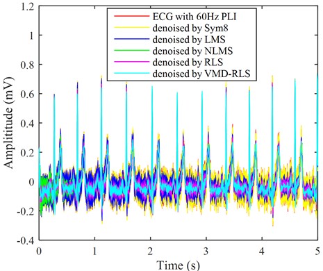
After the RLS and NLMS denoising methods were used to eliminate noise, the ECG signal basically returned to its original signal form, but there were still interference noises in the weak P wave, Q wave, S wave, and T wave regions. Especially during the first 0.5 s, the ECG signal that has been denoised by NLMS still exhibits significant interference noise. The ECG signal that has been denoised using the LMS and Sym8 denoising method, although some interference noise has been eliminated, still has significant interference noise. Especially in the weak P wave, Q wave, S wave, and T wave regions, the interference noise still overwhelms the characteristic signal.
Similar to the quantitative evaluation of high period white noise elimination, the SNR, RMSE and SD are used to measure the different effect of filtering and denoising between denoised signal and original signal. After experimental denoising, the denoising performance indicators of the five methods are shown in Table 2.
Table 2Comparisons of de-noising results of the five methods
Method | SNR (dB) | RMSE | SD |
Sym8 | 4.2251 | 9.9853e-04 | 0.1349 |
LMS | 7.6263 | 6.7500e-04 | 0.1245 |
NLMS | 15.0987 | 2.8555e-04 | 0.1166 |
RLS | 14.8611 | 2.9347e-04 | 0.1165 |
VMD-RLS | 26.7396 | 7.4754e-05 | 0.1149 |
The SNR after VMD-RLS denoising is the highest and the RMSE is the smallest, indicating the best performance. The minimum SD indicates that the more concentrated the distribution of signal values after denoising, the better the central tendency. After Sym8 denoising, the SNR is the smallest and RMSE is the largest, indicating that the denoising effect is the worst, and the SD is the largest, indicating that the signal value distribution after denoising is more scattered and the central tendency is worse. The SNR after NLMS denoising is close to twice that after LMS denoising, while the RMSE value is only about 0.4 of the latter, indicating that the denoising effect is significantly better than the latter. After RLS denoising, the SNR and SD are slightly lower than those after NLMS denoising, while the RMSE is slightly higher than the latter, indicating that the denoising effect is not as good as the latter, and the central tendency is slightly better than the latter. Compared to Table 1, it indicates that the five denoising methods may have slightly different denoising effects for different noise signals, but the denoising effect is still the best through VMD-RLS.
4. Conclusions
ECG belongs to weak electrical signals, and the collection process is easily affected by many external factors, including power frequency interference, electrode contact noise, and the physical condition of the subjects. As a result, these signals often contain significant noise, which complicates feature extraction and clinical diagnosis. A denoising method for ECG signals based on VMD and RLS is proposed to address the nonlinear and non-stationary characteristics of ECG signals. VMD is used to decompose ECG for artifact removal, and then RLS denoising is performed on the feature mode components after VMD. Finally, each modal component is reconstructed following denoising. This method has a good artifact removal effect, effectively avoiding the advantages of avoiding signal over decomposition and strong anti-modal aliasing ability.
The ECG signal denoising method based on Physionet ECG Database demonstrates the best denoising effect when compared to the RLS, LMS, and NLMS denoising methods. This approach effectively eliminates most of the noise while maintaining the characteristic form of the original signal. Additionally, the VMD-RLS algorithm has good convergence performance, with a faster convergence speed than the Sym8, RLS, LMS, and NLMS algorithms. It also exhibits low-weight offset noise and strong stability, making its filtering performance significantly superior to the other four methods.
This method demonstrates strong capabilities in modal recognition and denoising, offering improved efficiency and accuracy. It is beneficial for clinical real-time signal inspection and analysis, providing new insights into ECG signal denoising and enhancing support for the diagnosis and treatment of heart diseases. However, the denoising algorithm also has its shortcomings, such as the value for VMD decomposition needs to be determined in advance and cannot be adaptive. Additionally, the determination of other VMD parameters lacks a solid theoretical foundation and requires further refinement. Consequently, pursuing adaptive methods will be the next research direction for this study.
References
-
S. Chatterjee, R. S. Thakur, R. N. Yadav, L. Gupta, and D. K. Raghuvanshi, “Review of noise removal techniques in ECG signals,” IET Signal Processing, Vol. 14, No. 9, pp. 569–590, Dec. 2020, https://doi.org/10.1049/iet-spr.2020.0104
-
C. van Mieghem, M. Sabbe, and D. Knockaert, “The clinical value of the ECG in noncardiac conditions,” Chest, Vol. 125, No. 4, pp. 1561–1576, Apr. 2004, https://doi.org/10.1378/chest.125.4.1561
-
A. Lyon, A. Mincholé, J. P. Martínez, P. Laguna, and B. Rodriguez, “Computational techniques for ECG analysis and interpretation in light of their contribution to medical advances,” Journal of The Royal Society Interface, Vol. 15, No. 138, p. 20170821, Jan. 2018, https://doi.org/10.1098/rsif.2017.0821
-
M. Merone, P. Soda, M. Sansone, and C. Sansone, “ECG databases for biometric systems: A systematic review,” Expert Systems with Applications, Vol. 67, pp. 189–202, Jan. 2017, https://doi.org/10.1016/j.eswa.2016.09.030
-
L. Sörnmo, R. Bailón, and P. Laguna, “Spectral analysis of heart rate variability in time-varying conditions and in the presence of confounding factors,” IEEE Reviews in Biomedical Engineering, Vol. 17, pp. 322–341, Jan. 2024, https://doi.org/10.1109/rbme.2022.3220636
-
S. K. Mohapatra and M. N. Mohanty, “ECG analysis: a brief review,” Recent Advances in Computer Science and Communications, Vol. 14, No. 2, pp. 344–359, May 2021, https://doi.org/10.2174/2213275912666190408111123
-
A. Karimipour and M. R. Homaeinezhad, “Real-time electrocardiogram P-QRS-T detection-delineation algorithm based on quality-supported analysis of characteristic templates,” Computers in Biology and Medicine, Vol. 52, pp. 153–165, Sep. 2014, https://doi.org/10.1016/j.compbiomed.2014.07.002
-
O. Durgesh Kumar and M. Subashini, “Analysis of electrocardiograph (ECG) signal for the detection of abnormalities using Matlab,” International Journal of Biomedical and Biological Engineering, Vol. 8, No. 2, pp. 120–123, Feb. 2014, https://doi.org/10.5281/zenodo.1091402
-
M. A. Serhani, H. T. El Kassabi, H. Ismail, and A. Nujum Navaz, “ECG monitoring systems: review, architecture, processes, and key challenges,” Sensors, Vol. 20, No. 6, p. 1796, Mar. 2020, https://doi.org/10.3390/s20061796
-
H. Y. Mir and O. Singh, “ECG denoising and feature extraction techniques – a review,” Journal of Medical Engineering and Technology, Vol. 45, No. 8, pp. 672–684, Nov. 2021, https://doi.org/10.1080/03091902.2021.1955032
-
S. A. Taouli and F. Bereksi-Reguig, “Noise and baseline wandering suppression of ECG signals by morphological filter,” Journal of Medical Engineering and Technology, Vol. 34, No. 2, pp. 87–96, Dec. 2009, https://doi.org/10.3109/03091900903336886
-
I. I. Christov and I. K. Daskalov, “Filtering of electromyogram artifacts from the electrocardiogram,” Medical Engineering and Physics, Vol. 21, No. 10, pp. 731–736, Dec. 1999, https://doi.org/10.1016/s1350-4533(99)00098-3
-
G. Gao, Y. Zhong, Z. Gao, H. Zong, and S. Gao, “Maximum correntropy based spectral redshift estimation for spectral redshift navigation,” IEEE Transactions on Instrumentation and Measurement, Vol. 72, pp. 1–10, Jan. 2023, https://doi.org/10.1109/tim.2023.3275992
-
Y. Mao, Y. Zhong, Y. Gao, and Y. Wang, “A weak SNR signal extraction method for near-bit attitude parameters based on DWT,” Actuators, Vol. 11, No. 11, p. 323, Nov. 2022, https://doi.org/10.3390/act11110323
-
P. Madan, V. Singh, D. P. Singh, M. Diwakar, and A. Kishor, “Denoising of ECG signals using weighted stationary wavelet total variation,” Biomedical Signal Processing and Control, Vol. 73, p. 103478, Mar. 2022, https://doi.org/10.1016/j.bspc.2021.103478
-
A. Abdou and S. Krishnan, “Enhancement of single-lead dry-electrode ECG through wavelet denoising,” Frontiers in Signal Processing, Vol. 4, p. 2024, May 2024, https://doi.org/10.3389/frsip.2024.1396077
-
N. Mourad, “ECG denoising algorithm based on group sparsity and singular spectrum analysis,” Biomedical Signal Processing and Control, Vol. 50, pp. 62–71, Apr. 2019, https://doi.org/10.1016/j.bspc.2019.01.018
-
M. R. Kose, M. K. Ahirwal, and R. R. Janghel, “Descendant adaptive filter to remove different noises from ECG signals,” International Journal of Biomedical Engineering and Technology, Vol. 33, No. 3, p. 258, Jan. 2020, https://doi.org/10.1504/ijbet.2020.107761
-
F. Mohaddes et al., “A pipeline for adaptive filtering and transformation of noisy left-arm ECG to its surrogate chest signal,” Electronics, Vol. 9, No. 5, p. 866, May 2020, https://doi.org/10.3390/electronics9050866
-
F. Wang, Q. Wang, F. Liu, J. Chen, L. Fu, and F. Zhao, “Improved NLMS-based adaptive denoising method for ECG signals,” Technology and Health Care, Vol. 29, No. 2, pp. 305–316, Mar. 2021, https://doi.org/10.3233/thc-202659
-
X. Liu, H. Wang, Z. Li, and L. Qin, “Deep learning in ECG diagnosis: A review,” Knowledge-Based Systems, Vol. 227, p. 107187, Sep. 2021, https://doi.org/10.1016/j.knosys.2021.107187
-
Y. Hou, R. Liu, M. Shu, X. Xie, and C. Chen, “Deep neural network denoising model based on sparse representation algorithm for ECG signal,” IEEE Transactions on Instrumentation and Measurement, Vol. 72, pp. 1–11, Jan. 2023, https://doi.org/10.1109/tim.2023.3251408
-
U. Satija, B. Ramkumar, and M. Sabarimalai Manikandan, “Noise‐aware dictionary‐learning‐based sparse representation framework for detection and removal of single and combined noises from ECG signal,” Healthcare Technology Letters, Vol. 4, No. 1, pp. 2–12, Feb. 2017, https://doi.org/10.1049/htl.2016.0077
-
K. Dragomiretskiy and D. Zosso, “Variational mode decomposition,” IEEE Transactions on Signal Processing, Vol. 62, No. 3, pp. 531–544, Feb. 2014, https://doi.org/10.1109/tsp.2013.2288675
-
J. Lian, Z. Liu, H. Wang, and X. Dong, “Adaptive variational mode decomposition method for signal processing based on mode characteristic,” Mechanical Systems and Signal Processing, Vol. 107, pp. 53–77, Jul. 2018, https://doi.org/10.1016/j.ymssp.2018.01.019
-
R. Djemili and I. Djemili, “Nonlinear and chaos features over EMD/VMD decomposition methods for ictal EEG signals detection,” Computer Methods in Biomechanics and Biomedical Engineering, Vol. 27, No. 15, pp. 2091–2110, Nov. 2024, https://doi.org/10.1080/10255842.2023.2271603
-
S. Parri, K. Teeparthi, and V. Kosana, “A hybrid VMD based contextual feature representation approach for wind speed forecasting,” Renewable Energy, Vol. 219, p. 119391, Dec. 2023, https://doi.org/10.1016/j.renene.2023.119391
-
S. N. Makhadmeh et al., “Recent advances in Grey Wolf optimizer, its versions and applications: review,” IEEE Access, Vol. 12, pp. 22991–23028, Jan. 2024, https://doi.org/10.1109/access.2023.3304889
-
S. Behera, M. N. Mohanty, and S. K. Mohapatra, “Design of optimized adaptive filter for artifact removal from EEG signal,” Journal of Statistics and Management Systems, Vol. 26, No. 1, pp. 201–212, Jan. 2023, https://doi.org/10.47974/jsms-959
-
A. Y. Rahman, Mamba’Us Sa’Adah, and Istiadi, “Noise reduction in RTL-SDR using least mean square and recursive least square,” Jurnal RESTI (Rekayasa Sistem dan Teknologi Informasi), Vol. 4, No. 2, pp. 286–295, Apr. 2020, https://doi.org/10.29207/resti.v4i2.1667
-
R. Pande-Chhetri and A. Abd-Elrahman, “De-striping hyperspectral imagery using wavelet transform and adaptive frequency domain filtering,” ISPRS Journal of Photogrammetry and Remote Sensing, Vol. 66, No. 5, pp. 620–636, Sep. 2011, https://doi.org/10.1016/j.isprsjprs.2011.04.003
About this article

The authors thank the Natural Science Foundation of Fujian Province of China (2020J05212, 2022J011169), Education and Teaching Reform Research Project of Putian University (JG202391), and the Key technological innovation and industrialization projects in Fujian Province (2024XQ019).
The datasets generated during and/or analyzed during the current study are available from the corresponding author on reasonable request.
Chenhua Zhang: methodology, writing-review and editing. Wenjie Chen: data curation and software. Hongda Chen: formal analysis.
The authors declare that they have no conflict of interest.
