Modelling and optimization of the effect of rice husk ash on the California bearing ratio of Agbani soil using Scheffe’s method

2.1. Study area

The study area is situated in the south-eastern part of Nigeria in Agbani town, Enugu State. The soil was collected from the environs of the Enugu State University of Science and Technology (ESUT). The area is characterized by soil with considerable stiffness as observed by the difficulty posed during the excavation of the trial pit.

2.2. Sampling of materials

Trial pit for soil sampling was excavated, reaching a depth of 1.3 m with the use of shovels and pickaxe, the soil obtained were disturbed soil. Corresponding coordinates for the area was obtained using the Google Earth application. The Global positioning system (GPS) coordinate for the location is given as 6.304458° for latitude and 7.541142° for longitude respectively. The rice husk was sourced from a local rice miller located in Ugbawka, Nkanu East Local Government Area, Enugu State. Impurities present in the husks were sorted out; the husks were placed in bags and further transported to the laboratory where it was incinerated into ash.

2.3. Soil characterization method

The results from the laboratory testing of the soil informs its properties and aids its delineation based on those properties. The soil classification systems employed for the classification were the American Association of State Highway and Transport Officials (AASHTO) system and the Unified Soil Classification System. The soil in this study was classified based on these soil classification systems relative to the properties exhibited by the soil as observed from the laboratory test conducted [11-13].

2.4. Methods for testing of soil

The soil testing was carried out in harmony with the methods stipulated in BS 1377 (methods for soil testing). Therefore, to determine the index properties of the soil, the following tests that includes; Sieve analysis, Atterberg Limits, Compaction, Moisture Content, Specific Gravity and California Bearing Ratio were conducted. The standardized laboratory test results for the natural soil are highlighted in this paper. Methods of computation for some of the tests carried out are listed as Eq. (1) and Eq. (2):

where $w_1$ is the weight of dry soil and can, $w_2$ is the weight of wet soil and can, $w_3$ is the weight of can.

where LL is the liquid limit, PL is the plastic limit.

However, the property of the stabilized soil of keen interest in this study was the CBR property of the soil. The CBR test procedures is further discussed below.

2.5. Scheffe’s method of optimization

Henry Scheffe devised a method to optimize the behavior of stabilized soils, where the property to be improved depends on the percentages or proportions by weight of the constituents, not on their quantities in the combination. The responses known as “q, n-polynomials” are modelled using a second-degree polynomial regression. The method represents the inputs as a simplex, which is a polygon or factor space with a straight line as its basic simplex [14].

Straight lines signifies a one-dimensional factor spaces, solids are factor spaces that are three-dimensional such as; prisms, cones, tetrahedrons, spheres, cylinders, cubes, and cuboids, among other shapes [14].

In addition, based on the number of mix constituents that make up the factor space, the number of responses or observations to be expected is derived using Eq. (5):

Such that, $N$ is the number of observations required, $q$ is the Number of mixture components, $n$ is the Degree of the polynomials.

This research work involved a three-component mixture (Soil, RHA and Water) hence; the second-degree (3, 2) simplex model is a two-dimensional factor space represented as an Equilateral Triangle. Employing Eq. (5), to determine the number of responses in the experiment and control points. Hence:

Therefore, the mix design required six number of responses. In addition, six other responses were obtained for the control points used for validating the model. Furthermore, the response of the mixture is assumed a real value function on a simplex, to which an appropriate form of polynomial regression model is introduced.

The polynomial function of degree $n$ in $q$ variable has $C_{q+n}^n$ coefficients. If a mixture has a total of $q$ components and $K_i$ is the proportion of the $i$th component in the mixture such that $K_i\ge$ 0 ($i=$ 1, 2, …, $q$), then the summation of the component proportion is equal to one, i.e. $\mathrm{\Sigma }{K}_i-1=0$ [7-10].

Further written as:

One mix component appears at a single vertex of the simplex triangle. The simplex triangle’s vertices only contain stand-alone components of a mixture; blend components are limited to existing along the line that joins two vertices; and no more than two components of a mixture are present along a single line that joins two vertices concurrently.

2.5.1. Development of the model using Scheffe’s method

Scheffe’s design mix, which facilitated the formulation of the model, consists of two fundamental elements, which are the Pseudo and Real mix components, designated as $J$ and $K$, respectively. Scheffe states that the relationship between $J$ and $K$ is given as:

7

$\left[J\right]=\left[A\right]\left[K\right],$

where $\left[J\right]$ is the real mix ratio matrix, $\left[A\right]$ is the coefficient of the matrix, $\left[K\right]$ is the pseudo mix ratio matrix

The polynomial equation below is used to determine the system's response, which is represented by $Y:$

8

$Y=b_0+\mathrm{\Sigma }{b}_i{K}_i+\mathrm{\Sigma }{b}_{ij}{K}_i{K}_j+\mathrm{\Sigma }{b}_{ijk}{K}_i{K}_j{K}_k+\dots e.$

Considering a three component mix of two degrees, the response $Y$ is of the form:

9

$Y=b_0+\mathrm{\Sigma }{b}_i{K}_i+\mathrm{\Sigma }{b}_{ij}{K}_i{K}_j.$

Generally, the polynomial equation for a ternary system is given as:

10

$Y=b_0+b_1{K}_1+b_2{K}_2+b_3{K}_3+b_{11}{K}_{12}+b_{12}{K}_1{K}_2+b_{13}{K}_1{K}_3+b_{22}{K_2}^2+b_{23}{K}_2{K}_3+b_{33}{K_3}^2.$

Multiplying Eq. (6) by $b_0$:

11

$b_0=b_0{K}_1+b_0{K}_2+b_0{K}_3,$
$b_0=b_0\left(K_1+K_2+K_3\right).$

Furthermore, multiplying Eq. (6) by $K_1$, $K_2$ and $K_3$ successively and re-arranging gives:

12

${K_1}^2=K_1-K_1{K}_2-K_1{K}_3\to K_1={K_1}^2+K_1{K}_2+K_1{K}_3,$
${K_2}^2=K_2-K_1{K}_2-K_1{K}_3\to K_2={K_2}^2+K_1{K}_2+K_2{K}_3,$
${K_3}^2=K_3-K_1{K}_3-K_2{K}_3\to K_3={K_3}^2+K_1{K}_3+K_2{K}_3.$

Substituting Eq. (11) and Eq. (12) into Eq. (10) gives:

13

$Y=\left(b_0+b_1+b_{11}\right)K_1+\left(b_0+b_2+b_{22}\right)K_2+\left(b_0+b_3+b_{33}\right)K_3+\left(b_{12}-b_{11}-b_{22}\right)K_1{K}_2+\left(b_{13}-b_{11}-b_{33}\right)K_1{K}_3+\left(b_{23}-b_{22}-b_{33}\right)K_2{K}_3.$

Let:

14

${\beta }_i=b_0+b_1+b_{11},$

15

${\beta }_{ij}=b_{ij}–b_{ii}-b_{jj}.$

Re-writing Eq. (13) to arrive at a reduced second-degree polynomial with three variables:

16

$Y={\beta }_1{K}_1+{\beta }_2{K}_2+{\beta }_3{K}_3+{\beta }_{12}{K}_1{K}_2+{\beta }_{13}{K}_1{K}_3+{\beta }_{23}{K}_2{K}_3.$

Fig. 1Simplex triangle (2-dimensional factor space), where K1 is the Stand-alone of lateritic soil, K2 is the stand-alone of rice husk ash, K3 is the stand-alone of water, K12 is the blend of soil and rice husk ash, K13 is the blend of lateritic soil and water, K23 is the blend of rice husk ash and water

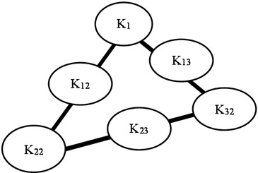
Therefore, Eq. (16) is the model as per Scheffe’s method of simplex lattice design used in this study for predicting the CBR values of the soil at various mix proportions. The coefficient of the second-degree polynomial is further derived from the vertex of the simplex triangle. As shown in Fig. 1, only stand-alone components are present at the vertex of the simplex triangle while intersections have blends of components. Hence, $K_1$, $K_2$ and $K_3$ have coordinates as follows: $K_1=\left(\mathrm{1,0},0\right)$; $K_2=\left(\mathrm{0,1},0\right)$; $K_3=\left(\mathrm{0,0},1\right)$.

2.6. Statistical validation technique for the model

The validity of the model was determined using a statistical test method to test the adequacy of the model and also enable for the acceptance of the study hypothesis.

3.1. Design mix matrix

A matrix is typically used to express the design mix's constituent. Additionally, as shown in Eq. (16), the optimization model is expressed in pseudo mix ratios, and Eq. (7) illustrates the link between the pseudo and real components.

By weighing the dry lateritic soil, the amount of rice husk ash was calculated, and the associated water content was determined. The mix ratios for the vertices where pure blends of the mix are to be present are as follows:

The related pseudo mix ratios have the shape of an identity matrix as follows:

Furthermore, Eq. (7) can be expressed as follows:

Substituting values for the matrix into Eq. (19) for the first run, the matrix becomes:

Eq. (20) gives the following coefficients for matrix $A$:

Considering the second run, the matrix is of the form:

Eq. (21) gives the following coefficients for matrix $A$:

For the third run, the matrix is of the form:

Eq. (22) gives the following coefficients for matrix $A$:

The coefficients derived from Eq. (20) to Eq. (22) put together, further yields the following coefficient matrix $A$:

3.2. Experimental results from the optimization

Sequel to the formulation of the design matrix using the Scheffe’s optimization technique and obtaining values for the mix proportion, the soil mix was subjected to California bearing ratio test for soaked condition, which was conducted on 12 (twelve) soil samples having distinct mix proportions. Six of which are trial mixes and the other six are control point mixes.

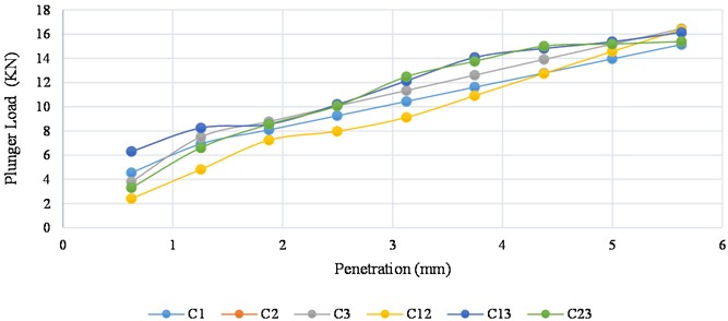
The results of the Soaked CBR for the treated soil samples are shown in the Tables 4 and 5, as well as the corresponding CBR plot for all responses are displayed in Fig. 3 and 4.

Fig. 2Graphical description of soaked CBR values

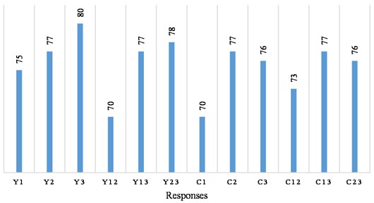
Fig. 3Experimental soaked CBR graph for trial mix responses

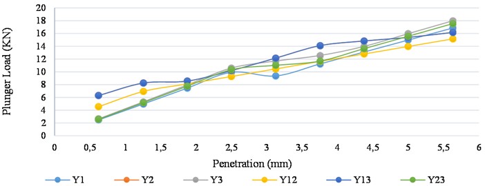
The CBR experimental values derived for each responses shows an increase in the experimental CBR values for the treated soil in comparison with the natural soil, which had a soaked CBR value of 70.14 %. The graphical representation from Fig. 2 shows that the mix design derived from the implementation of the Scheffe’s method gives a maximum soaked CBR value for the trial mix as 80 %, corresponding to the $Y_3$ response space and a maximum CBR value for the control point as 77 %, corresponding to the $C_2$ and $C_{13}$ response spaces.

Fig. 4Experimental soaked CBR graph for control mix responses

3.3. Model results

The computation of the results from the model formulated using Scheffe’s method was derived by substituting the values for the model coefficients, Pseudo components and further simplifying. The model equation stated in Eq. (16) as; $Y={\beta }_1{K}_1+{\beta }_2{K}_2+{\beta }_3{K}_3+{\beta }_{12}{K}_1{K}_2+{\beta }_{13}{K}_1{K}_3+{\beta }_{23}{K}_2{K}_3$. According to Scheffe, the values for ${\beta }_1$, ${\beta }_2$, and ${\beta }_3$ corresponds to, or are equal to the response values, $Y_1$, $Y_2$ and $Y_3$ respectively. Other model coefficients; ${\beta }_{12}$, ${\beta }_{13}$, and ${\beta }_{23}$ are derived using Eq. (18). Therefore, re-calling Eq. (17) and Eq. (18), the model coefficients are computed. The values computed are presented in Table 6.

Fig. 5Model and experimental results comparison

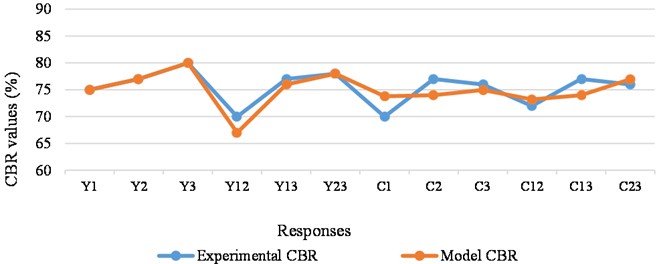
The values of the coefficients and corresponding pseudo component values are substituted into Eq. (16) to obtain the model equation for predicting the CBR values of the soil treated with RHA for soaked condition. The predictive model equation is derived as:

The predicted soaked CBR value is computed for each trial mix and control point using Eq. (33). The computation process is displayed in Table 7 and values are outlined for clarity in Table 8.

Fig. 5 displays a comparison between the experimental CBR values and the predicted values by the model. As seen in the Fig. 5, variations exist between both values as indicated by the displacements of the trend at specified responses. For responses $Y_1$, $Y_2$ and $Y_3$, the experimental and predicted values are exact as depicted on the graph. The extent of variance between the both values (experiment and model) is analyzed in the model validation process using statistical methods and insights is drawn on the predictive adequacy of the model formulated.

3.4. Model validation and analysis

The Null hypothesis, which states that; “there is no significant difference between the experimental CBR values and the model values”, as well as the Alternate hypothesis that states that; “there is a significant difference between the results of the experimental CBR and the model results”, were tested. The model validation was conducted using the 2016 version of the Microsoft Excel application software. The data analysis tool pack on the software was activated and used to run the F-test analysis. The results are shown in Table 9. Manual analysis of the F-test is further outlined in Appendix.

Results from the F-test gave the F-stat value for soaked CBR 4.34 with a corresponding F-critical value as 5.05. The F-test was conducted at a confidence level of 95 %. Therefore, with the value of the F-stat being less than the F-critical value, the result is indicative that the variance between the experimental CBR values and the Predicted values is insignificant.

In other words, there is no significant difference between the results of experimental CBR and the model predicted results. Hence, the null hypothesis is accepted and the model is adequate.