A cost model analysis in the process of refining petroleum using supplementary variable technique

S, Palaniammal; K, Kumar

doi:10.21595/mme.2025.24636

Mathematical Models in Engineering

Browse Journal

Submit article

Published: 09 March 2025

Check for updates

A cost model analysis in the process of refining petroleum using supplementary variable technique

Palaniammal S¹

Kumar K²

¹Department of Mathematics, Sri Krishna Adithya College of Arts and Science, Coimbatore, Tamilnadu, India

²Department of Science and Humanities, Sri Krishna College of Engineering and Technology, Coimbatore, Tamilnadu, India

Corresponding Author:

Palaniammal S

Cite the article Download PDF

Article in Press

Downloads 11

Abstract

This paper presents a cost model analysis for refining petroleum using an $M_{X} / G (a, b) / 1 .$ $M_{X} / G (a, b) / 1$ queuing system with two stages of heterogeneous services under steady-state conditions. The study derives the total average cost per unit time for two distinct service phases: Phase I and Phase II. In the first case, the analysis focuses on the total average cost of the system when the server operates in Phase I with a probability of $(π_{1})$ at any given time, and in Phase II with a probability of $(π_{2})$ . Additionally, the model incorporates holding costs, operating costs, renovation costs for both phases, and closure time costs. Finally, numerical tables and graphical representations are provided to illustrate the observations regarding the total average cost, renovation rate, and arrival rate.

Highlights

Threshold Value vs. Total Average Cost
Breakdown Value vs. Total Average Cost
Renovation rate vs. Total Average Cost
Performance measurements vs. Arrival rate
Performance measurements vs. Arrival rate

1. Introduction

In the literature on queueing systems, only a few authors have specifically addressed breakdown repairs or renovations at service stations. In practice, service stations often require renovations due to breakdowns, which significantly impact the system, particularly the queue length, server busy periods, and customer waiting times. Wang et al. [4] optimized the M/G/1 queue with a T-policy, accounting for server failures and typical startup durations using various system performance metrics. Choudhury and Tadj [4] examined an M/G/1 queue with two service phases, focusing on server failures and delayed repairs. Their work generalized both the traditional M/G/1 queue with random breakdowns and delayed repairs, as well as the M/G/1 queue with a second optional service and server breakdowns. Jain and Agrawal [3] investigated optimal strategies for bulk queues with different types of server breakdowns, assuming that breakdowns occur only when the server is active and require a random, limited number of repair steps.

This is the first study to analyze a two-stage heterogeneous queueing system with generally distributed variable batch size service and bulk arrivals. Notably, in the existing literature on two-stage heterogeneous queueing models, only bulk arrivals have been considered, with no studies addressing bulk service in such systems. This gap in the literature inspired the development of this paper. Our study stands out in several ways: it introduces a variable batch size service queueing model, which has greater practical relevance, within the framework of a two-stage heterogeneous system. Additionally, using Lee's method, we derive the probability generating function for the queue length distribution at any given time epoch under steady-state conditions.

This paper aims to discuss the following comparisons: the threshold value against the overall average cost and performance metrics, the probability of breakdown against the overall average cost and performance metrics, the renovation rate versus the overall average cost and performance metrics, and the arrival rate versus the performance metrics.

2. Model description and system equations

The single server architecture is used in a real-world setting during the refining of crude oil. There are several organic molecules in petroleum. Refining petroleum is the process of removing impurities and separating its components into usable products.

The refining process consists of two service phases: Phase I focuses on separating water and removing sulfur compounds, while Phase II involves the fractionation process.

Crude oil is a stable mixture of oil and saltwater. In Phase I, a significant volume of crude oil is passed between two highly charged electrodes to remove the saltwater. The water droplets are vaporized and separated. The water-free oil is then treated with copper oxide, which reacts with sulfur-containing compounds in the petroleum to form a copper sulfide precipitate in the reactor (Server I). In Phase II, this precipitate is removed through filtration.

In Phase II, the majority of the crude oil is heated in a furnace to a temperature of 400 degrees Celsius, causing all components except the asphalt residue cake to vaporize. The vapor passes through the fractionation column (Server II), a tall, cylindrical tower containing multiple horizontal stainless steel trays. Each tray is equipped with a chimney covered by a loose cap. In the fractionation process, trays at lower levels handle components with high boiling points, while trays at higher levels handle those with low boiling points. This process yields uncondensed gas and petroleum products such as naphtha, kerosene, diesel oil, heavy oil, and road tar. If either Server I or Server II experiences a malfunction, the renovation process is initiated immediately. Once the renovation is complete, normal service resumes.

Before leaving, the operator must complete tasks such as cleaning and inspecting the tools. Upon returning to the crude petroleum refining process, if the available crude oil quantity is less than the required batch size, the operator focuses on other tasks until a sufficient quantity is available.

The described process can be modeled as an $M_{X} / G (a, b) / 1$ queueing system with two stages of heterogeneous service and server breakdowns. Arrivals follow a Poisson process with an arrival rate $ƛ$ . The server activates to provide service to a batch of size $m i n (ξ, b)$ customers, where $b \geq a$ , once it detects at least $a$ customers are waiting in the queue. The service consists of two consecutive phases: Phase I (FPS) and Phase II (SPS), both operating under a First-Come-First-Served (FCFS) discipline. Service times are assumed to follow general distributions with a specified probability density function (PDF).

The server is subject to breakdowns during both service phases, with a breakdown probability of $(π_{1})$ during Phase I and $(π_{2})$ during Phase II. In the event of a breakdown in any phase, the server is immediately sent for repairs. Once repaired, the server resumes service for the remaining customers in the batch.

After completing each SPS, the server performs closedown tasks during its closedown time (C). If the queue length is less than $a$ , the server takes a series of random-length vacations. Otherwise, it continues to serve the next batch.

2.1. Notations and assumptions

This work employs the following notations.

$ƛ$ is the arrival rate , let $μ_{1}$ and $μ_{1}$ represent the service rate during peak periods in phases I and II respectively, $X (z_{1})$ is the PGF of $X$ , which is the group size random variable, and is the probability that $X = k$ . Assume that S1(.), S2(.), R1(.), R2(.), and V(.) represent the CDF of service time in phase I, services time in phase II, renovation time in phase I, renovation time in phase II, and vacation time, respectively, define ${S^{0}}_{1} (t_{1}), {S^{0}}_{2} (t_{1}), {R^{0}}_{1} (t_{1}), {R^{0}}_{2} (t_{1})$ and $V^{0} (t_{1})$ as the remaining service time in regular period in phase I of a batch time at time $t_{1}$ , remaining service time in regular period in phase II of a batch time at time $t_{1}$ , remaining renovation time in phase I and phase II respectively and denote ${\tilde{S}}_{1} (θ_{1})$ , ${\tilde{S}}_{2} (θ_{1})$ , ${\tilde{R}}_{1} (θ_{1})$ , ${\tilde{R}}_{2} (θ_{1})$ , and $\tilde{V} (θ_{1})$ the LST of $S_{1}$ , $S_{2}$ , $R_{1}$ , $R_{2}$ and $V$ respectively.

$N_{q_{1}} (t_{1})$ – size of the queue at time $t_{1}$ .

$N_{s_{1}} (t_{1})$ – customers using the service at the moment $t_{1}$ .

$Y_{1} (t_{1})$ = 0 – whenever the server is away; = 1 if the server is performing phase I service while being busy; = 2 if the server is performing phase II service while being busy; = 3 if the server is undergoing initial step of renovation; = 4 if the server is undergoing final step of renovation; = 5 if the server is performing a shutdown task.

$Z_{1} (t_{1})$ = $j$ if the server is taking a vacation, it will begin during the idle period.

3. PGF of the queue size at different epochs

(a) Close down completion epoch:

1

C (z_{1}) = \frac{(\tilde{C} (ƛ - ƛ X (z_{1})) - 1) \sum_{i = 0}^{a - 1} P_{i}^{(2)} {z_{1}}^{i}}{(- ƛ + ƛ X (z_{1}))} .

(b) Vacation completion epoch:

2

V (z_{1}) = \frac{(\tilde{V} (ƛ - ƛ X (z_{1})) - 1) [\tilde{C} (ƛ - ƛ X (z_{1})) \sum_{i = 0}^{a - 1} P_{i}^{(1)} z^{i} + \sum_{i = 0}^{a - 1} q_{i} {z_{1}}^{i}]}{(- ƛ + ƛ X (z_{1}))} .

(c) Service in phase I completion epoch:

3

P_{1} (z_{1}) = \frac{\{\begin{matrix} ({\tilde{S}}_{1} (ƛ - ƛ X (z_{1})) - 1) \sum_{i = a}^{b - 1} (P_{i}^{(1)} ({z_{1}}^{b} - {z_{1}}^{i}) + R_{i}^{(1)} ({z_{1}}^{b} - {z_{1}}^{i}) + q_{i} ({z_{1}}^{b} - {z_{1}}^{i})) \\ + ({\tilde{S}}_{1} (ƛ - ƛ X (z_{1})) - 1) \tilde{V} (ƛ - ƛ X (z_{1})) \tilde{C} ((ƛ - ƛ X (z_{1})) - 1) \sum_{i = 0}^{a - 1} P_{i}^{(1)} {z_{1}}^{i} \\ + ({\tilde{S}}_{1} (ƛ - ƛ X (z_{1})) - 1) (\tilde{V} (ƛ - ƛ X (z_{1})) - 1) \sum_{i = 0}^{a - 1} q_{i} {z_{1}}^{i} \end{matrix}\}}{\{\begin{matrix} (ƛ - ƛ X (z_{1})) ({1 + π}_{1} {\tilde{R}}_{1} (ƛ - ƛ X (z_{1})) - {π_{1} \tilde{S}}_{1} (ƛ - ƛ X (z_{1})) {\tilde{R}}_{1} (ƛ - ƛ X (z_{1}))) \\ \times {\tilde{R}}_{1} (ƛ - ƛ X (z_{1})) ({z_{1}}^{b} - {\tilde{S}}_{1} (ƛ - ƛ X (z_{1}))) \end{matrix}\}} .

(d) Service in phase II completion epoch:

4

P_{2} (z_{1}) = \frac{({\tilde{S}}_{2} (ƛ - ƛ X (z_{1})) - 1) \sum_{i = a}^{b - 1} (P_{i}^{(2)} ({z_{1}}^{b} - {z_{1}}^{i}) + R_{i}^{(2)} ({z_{1}}^{b} - {z_{1}}^{i}) + P_{0}^{(1)} ({z_{1}}^{b} - {z_{1}}^{i}))}{\{\begin{matrix} (ƛ - ƛ X (z_{1})) ({1 + π}_{2} {\tilde{R}}_{2} (ƛ - ƛ X (z_{1})) - {π_{2} \tilde{S}}_{2} (ƛ - ƛ X (z_{1})) {\tilde{R}}_{2} (ƛ - ƛ X (z_{1}))) \\ \times ({z_{1}}^{b} - {\tilde{S}}_{2} (ƛ - ƛ X (z_{1}))) \end{matrix}\}} .

(e) Renovation in phase I completion epoch:

5

R_{1} (z_{1}) = \frac{\{\begin{matrix} π_{1} ({\tilde{R}}_{1} (ƛ - ƛ X (z_{1})) - 1) ({\tilde{S}}_{1} (ƛ - ƛ X (z_{1})) - 1) \\ \times \sum_{i = a}^{b - 1} (P_{i}^{(1)} ({z_{1}}^{b} - {z_{1}}^{i}) + R_{i}^{(1)} ({z_{1}}^{b} - {z_{1}}^{i}) + q_{i} ({z_{1}}^{b} - {z_{1}}^{i})) \\ + π_{1} ({\tilde{R}}_{1} (ƛ - ƛ X (z_{1})) - 1) ({\tilde{S}}_{1} (ƛ - ƛ X (z_{1})) - 1) \\ \times \tilde{V} (ƛ - ƛ X (z_{1})) \tilde{C} ((ƛ - ƛ X (z_{1})) - 1) \sum_{i = 0}^{a - 1} P_{i}^{(1)} {z_{1}}^{i} \\ + π_{1} ({\tilde{R}}_{1} (ƛ - ƛ X (z_{1})) - 1) ({\tilde{S}}_{1} (ƛ - ƛ X (z_{1})) - 1) (\tilde{V} (ƛ - ƛ X (z_{1})) - 1) \sum_{i = 0}^{a - 1} q_{i} {z_{1}}^{i} \end{matrix}\}}{\{\begin{matrix} (ƛ - ƛ X (z_{1})) ({1 + π}_{1} {\tilde{R}}_{1} (ƛ - ƛ X (z_{1})) - {π_{1} \tilde{S}}_{1} (ƛ - ƛ X (z_{1})) {\tilde{R}}_{1} (ƛ - ƛ X (z_{1}))) \\ \times {\tilde{R}}_{1} (ƛ - ƛ X (z_{1})) ({z_{1}}^{b} - {\tilde{S}}_{1} (ƛ - ƛ X (z_{1}))) \end{matrix}\}} .

(f) Renovation in phase II completion epoch:

6

R_{2} (z_{1}) = \frac{\begin{matrix} π_{2} ({\tilde{R}}_{2} (ƛ - ƛ X (z_{1})) - 1) ({\tilde{S}}_{2} (ƛ - ƛ X (z_{1})) - 1) \\ \times \sum_{i = a}^{b - 1} (P_{i}^{(2)} ({z_{1}}^{b} - {z_{1}}^{i}) + R_{i}^{(2)} ({z_{1}}^{b} - {z_{1}}^{i}) + P_{0}^{(1)} ({z_{1}}^{b} - {z_{1}}^{i})) \end{matrix}}{\{\begin{matrix} (ƛ - ƛ X (z_{1})) ({1 + π}_{1} {\tilde{R}}_{1} (ƛ - ƛ X (z_{1})) - {π_{1} \tilde{S}}_{1} (ƛ - ƛ X (z_{1})) {\tilde{R}}_{1} (ƛ - ƛ X (z_{1}))) \\ \times {\tilde{R}}_{1} (ƛ - ƛ X (z_{1})) ({z_{1}}^{b} - {\tilde{S}}_{1} (ƛ - ƛ X (z_{1}))) \end{matrix}\}} .

4. Some important performance measures

Expected length of busy period:

7

E (B) = \frac{(E (T_{1}) + E (T_{2}))}{\sum_{i = 0}^{a - 1} d_{i},} E (T_{1}) = E (S_{1}) + π_{1} E (R_{1}), E (T_{2}) = E (S_{2}) + π_{2} E (R_{2}) .

Expected length of the idle period:

8

E (I) = E (I_{1}) + E (C),

E (I_{1}) = \frac{E (V)}{1 - \sum_{n = 0}^{a - 1} Q_{1 n} (0)} = \frac{E (V)}{1 - \sum_{n = 0}^{a - 1} \sum_{i = 0}^{n} \{\sum_{j = 0}^{n - 1} α_{j} β_{n - i - j}\} P_{i}^{(1)}},

where $I_{1}$ is the random variable denoting the “Idle period due to multiple vacation process”, $E (C)$ is the expected closedown time.

Expected queue length at an arbitrary time epoch:

9

E (Q) = \frac{\{\begin{matrix} ({(b - s_{21})}^{2} H_{11} + {(b - s_{21})}^{2} {(b - s_{11})}^{2} V_{11}) \sum_{i = 0}^{a - 1} P_{i}^{(1)} \\ + ({(b - s_{21})}^{2} H_{12} - {(b - s_{21})}^{2} {(b - s_{11})}^{2} V_{12}) \sum_{n = 0}^{a - 1} i P_{i}^{(1)} \\ + {(b - s_{21})}^{2} {(b - s_{11})}^{2} L_{1} \sum_{i = 0}^{a - 1} P_{i}^{(2)} + {(b - s_{21})}^{2} {(b - s_{11})}^{2} L_{2} \sum_{n = 0}^{a - 1} {i P}_{i}^{(2)} \\ + ({(b - s_{21})}^{2} H_{13} + {(b - s_{21})}^{2} {(b - s_{11})}^{2} V_{13}) \sum_{i = 0}^{a - 1} q_{i} \\ + ({(b - s_{21})}^{2} H_{14} - {(b - s_{21})}^{2} {(b - s_{11})}^{2} V_{14}) \sum_{n = 0}^{a - 1} i q_{i} \\ + {(b - s_{21})}^{2} H_{15} \sum_{i = a}^{b - 1} (b - i) C_{i}^{(1)} + {(b - s_{21})}^{2} H_{16} \sum_{i = a}^{b - 1} (b (b - 1) - i (i - 1)) C_{i}^{(1)} \\ {+ (b - s_{21})}^{2} H_{25} \sum_{i = a}^{b - 1} (b - i) (C_{i}^{(2)} + P_{0}) + {(b - s_{11})}^{2} H_{26} \\ \times \sum_{i = a}^{b - 1} (b (b - 1) - i (i - 1)) (C_{i}^{(2)} + P_{0}) \end{matrix}\}}{2 {(ƛ X_{1})}^{2} {(b - s_{11})}^{2} {(b - s_{21})}^{2}},

H_{11} = 2 π_{1} T_{11} S_{11} R_{11} (V_{1} + C_{1}) + T_{11} S_{11} (V_{2} + C_{2} + 2 V_{1} C_{1}) - 2 T_{11} S_{12} (V_{1} + C_{1}),

H_{12} = T_{11} S_{11} (V_{1} + C_{1}), H_{13} = 2 π_{1} T_{11} S_{11} R_{11} V_{1} + T_{11} S_{11} V_{2} - 2 T_{11} S_{12} V_{1},

H_{14} = T_{11} S_{11} V_{1}, H_{15} = 2 π_{1} T_{11} S_{11} R_{11} - 2 T_{11} S_{11}, H_{16} = T_{11} S_{11},

T_{11} = (ƛ X_{1}) (b - s_{11}), H_{25} = 2 π_{1} T_{21} S_{21} R_{21} - 2 T_{21} S_{22}, H_{26} = T_{21} S_{21},

T_{21} = (ƛ X_{1}) (b - s_{21}), V_{11} = (V_{1} (ƛ X_{2}) - 2 V_{2} (ƛ X_{1})), V_{12} = 2 V_{1} (ƛ X_{1}),

V_{13} = V_{1} (ƛ X_{2}), V_{14} = 2 V_{1} (ƛ X_{1}), L_{1} = ((ƛ X_{1}) C_{2} - (ƛ X_{2}) C_{1}), L_{1} = 2 (ƛ X_{1}) C_{1} .

Expected waiting time:

10

E (W) = \frac{E (Q)}{ƛ E (X)} .

5. Cost model

We begin by making the following assumptions to generate the expression for calculating the total average cost: Let $C_{s}$ be the initial start up cost, $C_{h}$ represent the holding expense per client, $C_{0}$ represent the operating cost per hour, $C_{r}$ represent the prize for each unit of vacation time, $C_{r p 1}$ represent the phase I renovation cost per unit of time, $C_{r p 2}$ represent the phase II renovation cost per unit of time, and $C_{u}$ represent the time-per-closedown cost. The cycle’s length is calculated by adding the busy and idle periods. Now, the expected length of cycle $E (T_{c})$ , is obtained as:

11

E (T_{c}) = E (I) + E (B) = \frac{E (V)}{P (U = 0)} + E (C) + \frac{(E (S_{1}) + E (S_{2}))}{\sum_{i = 0}^{a - 1} P_{i}^{(1)}} .

The Total average cost per unit is given by.

Total average cost = Start-up cost per cycle + Renovation cost per cycle in phase I and phase II + Holding cost of customer in the queue + Operating cost * $ρ$ + Closedown time cost – Reward due to Vacation per cycle.

Total average cost:

12

[C_{s} + (C_{r p 1} + C_{r p 2}) \frac{E (R) E (B)}{E (T)} - C_{r} \frac{E (V)}{P (U = 0)} + C_{u} E (C)] \frac{1}{E (T_{c})} + C_{h} E (Q) + C_{0} (ρ),

where, $ρ = ƛ^{2} {(E (X))}^{2} [E (S_{1}) + π E (R_{1})] [E (S_{2}) + π E (R_{2})] / b$ .

In the section below, we provide a few numerical examples to further clarify the aforementioned answer.

6. A numerical example

Numerical methods are used to calculate the queue size distribution’s unknown probability.

The zeros of the function in Matlab ${z_{1}}^{b} - (1 - π) {\tilde{S}}_{1} (ƛ - ƛ X (z_{1})) - π {\tilde{S}}_{2} (ƛ - ƛ X (z_{1})) \tilde{R} (ƛ - ƛ X (z_{1}))$ are discovered, and several simultaneous equations are resolved.

The following suppositions are used to analyse a numerical model.

The arrival batch size distribution has a mean of 2 and a geometric standard deviation of 2 - Erlangen, Phase I and Phase II vacation, shutdown, and renovation times are exponential with parameters $α =$ 10, $β =$ 8, $γ_{1} =$ 7 and $γ_{2} =$ 7 respectively, $π_{1} =$ 0.2 and $π_{2} =$ 0.4.

(i) Start-up costs = ₹.4.

(ii) Holding costs = ₹.0.50 / customer.

(iii) Operating costs = ₹.5 / unit time.

(iv) Reward due to vacation = ₹.2 / unit time.

(v) Renovation cost in phase I = ₹.0.4 / unit time.

(vi) Renovation cost in phase II = ₹.0.5 / unit time.

(vii) Closure time cost = ₹.0.25 / unit time.

7. Effect of cost averages and threshold values

We have numerically examined the model to show the effects of the suggested model.

In refining of crude petroleum process, crude oil goes in bulk into the reactor (server I) for treating with copper oxide for forming copper sulphide precipitate following Poisson distribution, whose service follows an exponential distribution. 12 tons of crude oil can be handled by the reactor. After that, the bulk amount of crude oil with sulphide precipitate is heated upto 400 °C furnace. The vapor in bulk is passing through the fractionation column (server II) and it also following Poisson distribution, whose service is also follows an exponential distribution. When the operator completes the service and discovers that the number of tonnes available is below the threshold, he begins the closedown.

A $M_{X} / G (a, b) / 1$ queueing system with two stages of heterogeneous services, repeated vacations, and closedown with server breakdown can be used to model the system described above. Operating costs will be higher if the filter press starts with a threshold value of 2, which is the minimum capacity and higher yet if the threshold value is set at 12, which is the maximum capacity. We want to get the best threshold value.

Table 1Comparison of the threshold value to the overall average cost and performance metrics (Server breakdown) with ƛ= 4, μ1= 7, μ2= 9

A	$E_{x} (Q)$	$E_{x} (B)$	$E_{x} (I)$	$E_{x} (W)$	TAC
2	2.79	0.46	0.45	0.35	8.98
3	2.96	0.41	0.50	0.35	8.25
4	3.25	0.40	0.52	0.39	7.97
5	3.42	0.39	0.60	0.45	7.69
6	4.89	0.38	0.70	0.49	7.25
7	5.26	0.38	0.75	0.50	7.11
8	5.86	0.37	0.80	0.60	6.86
9	5.25	0.36	0.79	0.65	6.88
10	5.70	0.37	0.70	0.70	7.55
11	6.15	0.37	0.70	0.79	7.99
12	6.85	0.38	0.66	0.80	9.25

Table 2Comparison of the threshold value to the overall average cost and performance metrics (Server breakdown) with ƛ= 4, μ1= 7, μ2= 9

a	$E_{x} (Q)$	$E_{x} (B)$	$E_{x} (I)$	$E_{x} (W)$	TAC
2	2.58	0.36	0.47	0.30	8.26
3	2.76	0.34	0.55	0.32	7.63
4	3.02	0.34	0.63	0.35	7.04
5	3.32	0.33	0.71	0.39	6.60
6	3.66	0.33	0.78	0.43	6.32
7	4.02	0.33	0.78	0.48	6.20
8	4.41	0.33	0.84	0.53	6.20
9	4.83	0.34	0.83	0.58	6.30
10	5.28	0.34	0.83	0.63	6.47
11	5.77	0.34	0.83	0.70	6.70
12	6.31	0.34	0.82	0.76	6.98

It is clear that Table 1 shows that the management must set the minimum threshold value at 8 in a filter press for a vegetable oil refinery with a 12 ton per hour capacity in order to reduce the overall average cost.

Fig. 1Threshold value vs. total average cost

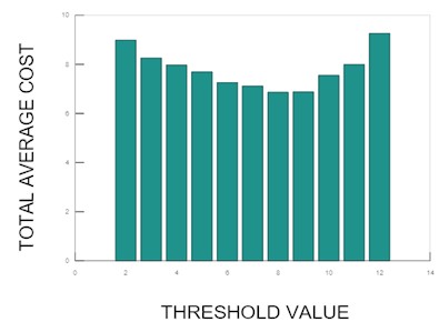
Fig. 2Threshold value vs. total average cost

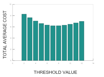
Table 3Comparison of the probability of breakdown value to the overall average cost and performance metrics

$π_{1}$	P	$E_{x} (Q)$	$E_{x} (B)$	$E_{x} (I)$	$E_{x} (W)$	TAC
0	0.74	5.78	1.78	0.96	1.60	10.30
0.1	0.76	6.23	1.88	0.96	1.65	10.34
0.2	0.79	6.74	2.00	0.95	1.72	10.42
0.3	0.81	7.33	2.14	0.95	1.79	10.53
0.4	0.83	8.60	2.30	0.95	1.88	10.70
0.5	0.85	8.79	2.50	0.95	1.97	10.94
0.6	0.88	9.73	2.75	0.94	2.09	11.26
0.7	0.90	10.87	2.06	0.94	2.23	11.69
0.8	0.92	12.30	3.45	0.94	2.41	12.27
0.9	0.95	14.12	3.97	0.94	2.64	13.07
1	0.97	16.57	4.68	0.93	2.95	14.19

Table 4Comparison of the probability of breakdown value to the overall average cost and performance metrics

$π_{2}$	$ρ$	$E_{x} (Q)$	$E_{x} (B)$	$E_{x} (I)$	$E_{x} (W)$	TAC
0	0.64	4.78	0.78	0.26	0.60	9.30
0.1	0.66	5.23	0.88	0.26	0.65	9.35
0.2	0.69	5.74	1.00	0.25	0.72	9.42
0.3	0.71	6.33	1.14	0.25	0.79	9.54
0.4	0.73	7.60	1.30	0.25	0.88	9.71
0.5	0.75	7.79	1.50	0.25	0.97	9.94
0.6	0.78	8.73	1.75	0.24	1.09	10.26
0.7	0.80	9.87	1.06	0.24	1.23	10.69
0.8	0.82	11.29	2.45	0.24	1.41	11.28
0.9	0.85	13.11	2.97	0.24	1.64	12.08
1	0.87	15.56	3.68	0.23	1.95	13.20

Table 5Renovation rate vs overall average cost and performance metrics

$β_{1}$	P	$E_{x} (Q)$	$E_{x} (B)$	$E_{x} (I)$	$E_{x} (W)$	TAC
1	0.96	35.92	13.08	0.23	13.36	40.20
2	0.80	12.26	1.98	0.24	1.53	14.20
3	0.75	8.19	1.41	0.25	1.02	10.36
4	0.72	6.91	1.21	0.25	0.86	9.84
5	0.70	6.31	1.10	0.25	0.79	9.61
6	0.69	5.96	1.04	0.25	0.75	9.49
7	0.69	5.74	1.00	0.25	0.72	9.42
8	0.68	5.59	0.97	0.26	0.70	9.38
9	0.68	5.48	0.94	0.26	0.68	9.34

Table 6Renovation rate vs overall average cost and performance metrics

$β_{2}$	$ρ$	$E_{x} (Q)$	$E_{x} (B)$	$E_{x} (I)$	$E_{x} (W)$	TAC
1	0.96	36.92	13.08	0.23	13.36	41.20
2	0.80	12.26	1.98	0.24	1.54	12.20
3	0.75	8.19	1.41	0.25	1.02	10.36
4	0.72	6.91	1.21	0.25	0.86	9.84
5	0.70	6.31	1.10	0.25	0.79	9.61
6	0.69	5.96	1.04	0.25	0.75	9.49
7	0.69	5.74	1.00	0.25	0.71	9.42
8	0.68	5.59	0.97	0.26	0.70	9.38
9	0.68	5.48	0.94	0.26	0.69	9.34

Fig. 3Breakdown value vs. total average cost

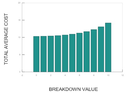
Fig. 4Breakdown value vs. total average cost

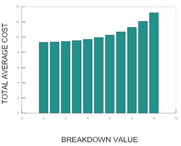
Fig. 5Renovation rate vs. total average cost

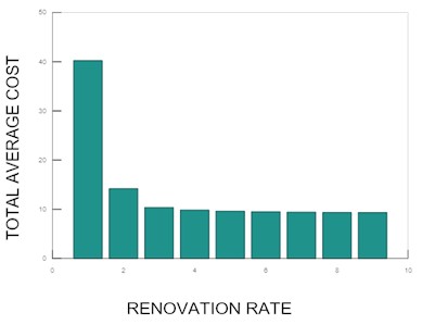
Fig. 6Renovation rate vs. total average cost

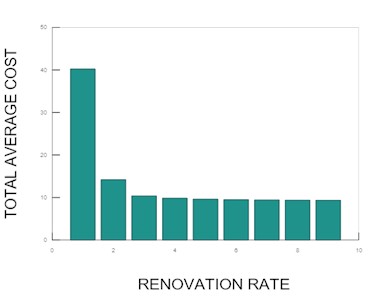
From Table 4, Figs. 4 and 5 it has been noticed that the server’s busiest time grows as the rate of renovation does. and $E (Q)$ reduce.

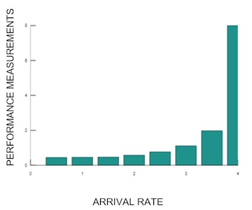
8. Comparison of the arrival rate and performance metrics

The expected queue length $(Q)$ , expected idle period length $E (I)$ , expected busy period length $E (B)$ , and expected waiting time $E (W)$ are computed for a variety of arrival rates and a variety of service rates and are shown in Tables 1-5. Assuming that $a =$ 2, $b =$ 5, $ƛ$ = 4 and $μ =$ 5.

Tables 5 to 9 show that as arrival rates rise, so does the anticipated queue length $E (Q)$ (refer columns 1 and 3 of each table). However, for a specific arrival rate, projected queue length decreases as service rate rises (considering the entire tables together). For instance, if the service rate is 2.0, then we have $E (Q)$ = 0.6331 for 0.5 (see Table 5). As opposed to $E (Q)$ = 0.4203 for = 0.5 when service rate = 4.0 (see Table 9). Similar findings are also seen for the performance indicators $E (B)$ , $E (I)$ , and $E (W)$ . In fact, these patterns reflect the effectiveness of conventional queuing models.

Table 7Performance measurements vs arrival rate (μ= 2)

$ƛ$	P	$E_{x} (Q)$	$E_{x} (B)$	$E_{x} (I)$	$E_{x} (W)$
0.5	0.17	0.53	1.91	0.28	0.53
1	0.33	1.18	2.13	0.27	0.59
1.5	0.50	2.41	2.31	0.26	0.80
2	0.66	5.00	3.15	0.25	1.25
0.5	0.17	0.53	1.91	0.28	0.53
1	0.33	1.18	2.13	0.27	0.59

Table 8Performance measurements vs arrival rate (μ= 2.5)

$ƛ$	P	$E_{x} (Q)$	$E_{x} (B)$	$E_{x} (I)$	$E_{x} (W)$
0.5	0.21	0.63	2.80	0.27	0.63
1	0.41	1.65	3.96	0.25	0.82
1.5	0.62	4.04	4.26	0.25	1.35
2	0.82	12.19	8.74	0.23	3.05

Fig. 7Performance measurements vs. arrival rate

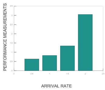
Fig. 8Performance measurements vs. arrival rate

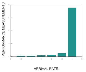
Table 9Performance measurements vs arrival rate (μ= 3)

$ƛ$	P	$E_{x} (Q)$	$E_{x} (B)$	$E_{x} (I)$	$E_{x} (W)$
0.5	0.14	0.48	1.84	0.29	0.48
1	0.28	0.94	1.98	0.28	0.48
1.5	0.42	1.74	2.15	0.28	0.58
2	0.56	3.13	2.21	0.26	0.78
2.5	0.70	5.86	2.48	0.25	1.17
3	0.83	13.22	4.46	0.24	2.20
3.5	0.97	97.48	27.64	0.23	13.93

Table 10Performance measurements vs arrival rate (μ= 3.5)

$ƛ$	P	$E_{x} (Q)$	$E_{x} (B)$	$E_{x} (I)$	$E_{x} (W)$
0.5	0.12	0.44	1.76	0.32	0.44
1	0.24	0.81	1.85	0.30	0.45
1.5	0.36	1.39	1.95	0.29	0.46
2	0.48	2.30	2.13	0.28	0.57
2.5	0.60	3.81	2.59	0.26	0.76
3	0.72	6.66	3.05	0.25	1.11
3.5	0.84	13.81	3.52	0.24	1.97
0.5	0.12	0.44	1.76	0.32	0.44

Fig. 9Performance measurements vs. arrival rate

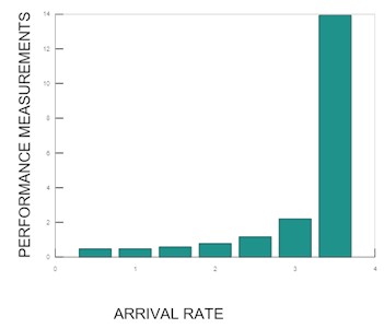
Fig. 10Performance measurements vs. arrival rate

9. Conclusions

In this study, we analyze the behavior of server failures without interruption in an $M_{X} / G (a, b) / 1$ queueing system with two phases of heterogeneous service. We derive the probability generating function for the queue size at any given time epoch and at various completion epochs, and calculate several important performance indicators. The numerical results obtained support the theoretical development of the model. A pricing model is also proposed, along with a specific example of the model. The numerical outcomes indicate that, as a result of server breakdowns, the expected queue length, the server’s busy period, and the customers’ waiting times all increase, while the server’s idle period decreases. Furthermore, it is observed that as the renovation rate increases, the expected queue duration decreases.

References

B. T. Doshi, “Queueing systems with vacations? A survey,” Queueing Systems, Vol. 1, pp. 29–66, Jun. 1986, https://doi.org/10.1007/bf01149327

Publisher
H. S. Lee, “Steady state probabilities for the server vacation model with group arrivals and under control operation policy,” Journal of the Korean Operations Research and Management Science Society, Vol. 16, pp. 36–48, 1991.

Search CrossRef
H. Takagi, Queueing Analysis: “A Foundation of Performance Evaluation, Vol. I: Vacations and Priority Systems”. Elsevier, 1991.

Search CrossRef
K. C. Madan, “An M/G/1 queue with second optional service,” Queueing Systems, Vol. 34, No. 1/4, pp. 37–46, Jan. 2000, https://doi.org/10.1023/a:1019144716929

Publisher
K. C. Madan, “On a single server queue with two-stage heterogeneous service and deterministic server vacations,” International Journal of Systems Science, Vol. 32, No. 7, pp. 837–844, Jan. 2001, https://doi.org/10.1080/00207720121488

Publisher
J. Medhi, “A single server Poisson input queue with a second optional channel,” Queueing Systems, Vol. 42, No. 3, pp. 239–242, Jan. 2002, https://doi.org/10.1023/a:1020519830116

Publisher
K. C. Madan, W. Abu-Dayyeh, and M. Gharaibeh, “Steady state analysis of two Mx/M(a,b)/1 queue models with random breakdowns,” International Journal of Information and Management Sciences, Vol. 14, pp. 37–51, 2003.

Search CrossRef
R. Arumuganathan and S. Jeyakumar, “Steady state analysis of a bulk queue with multiple vacations, setup times with N-policy and closedown times,” Applied Mathematical Modelling, Vol. 29, No. 10, pp. 972–986, Oct. 2005, https://doi.org/10.1016/j.apm.2005.02.013

Publisher
K. C. Madan and G. Choudhury, “A single server queue with two phases of heterogeneous service under Bernoulli schedule and a general vacation time,” International Journal of Information and Management Sciences, Vol. 16, No. 2, 2005.

Search CrossRef
K.-H. Wang, T.-Y. Wang, and W. L. Pearn, “Optimal control of the N policy M/G/1 queueing system with server breakdowns and general startup times,” Applied Mathematical Modelling, Vol. 31, No. 10, pp. 2199–2212, Oct. 2007, https://doi.org/10.1016/j.apm.2006.08.016

Publisher
G. Choudhury, L. Tadj, and M. Paul, “Steady state analysis of an Mx/G/1 queue with two phase service and Bernoulli vacation schedule under multiple vacation policy,” Applied Mathematical Modelling, Vol. 31, No. 6, pp. 1079–1091, Jun. 2007, https://doi.org/10.1016/j.apm.2006.03.032

Publisher
T.-Y. Wang, K.-H. Wang, and W. L. Pearn, “Optimization of the T policy M/G/1 queue with server breakdowns and general startup times,” Journal of Computational and Applied Mathematics, Vol. 228, No. 1, pp. 270–278, Jun. 2009, https://doi.org/10.1016/j.cam.2008.09.021

Publisher
M. Jain and P. K. Agrawal, “Optimal policy for bulk queue with multiple types of server breakdown,” International Journal of Operational Research, Vol. 4, No. 1, pp. 35–54, Jan. 2009, https://doi.org/10.1504/ijor.2009.021617

Publisher
G. Choudhury, J.-C. Ke, and L. Tadj, “The N-policy for an unreliable server with delaying repair and two phases of service,” Journal of Computational and Applied Mathematics, Vol. 231, No. 1, pp. 349–364, Sep. 2009, https://doi.org/10.1016/j.cam.2009.02.101

Publisher
M. Jain and S. Upadhyaya, “Optimal repairable MX/G/1 queue with multi- optional services and Bernoulli vacation,” International Journal of Operational Research, Vol. 7, No. 1, p. 109, Jan. 2010, https://doi.org/10.1504/ijor.2010.029520

Publisher
V. Thangaraj S. Vanitha, “M/G/1 queue with two-stage heterogeneous service compulsory server vacation and random breakdowns,” International Journal of Contemporary Mathematical Sciences, Vol. 5, No. 7, pp. 307–322, 2010.

Search CrossRef
G. Choudhury, L. Tadj, and J.-C. Ke, “A two-phase service system with Bernoulli vacation schedule, setup time and N-policy for an unreliable server with delaying repair,” Quality Technology and Quantitative Management, Vol. 8, No. 3, pp. 271–284, Feb. 2016, https://doi.org/10.1080/16843703.2011.11673259

Publisher
M. Balasubramanian and R. Arumuganathan, “Steady state analysis of a bulk arrival general bulk service queueing system with modified M-vacation policy and variant arrival rate,” International Journal of Operational Research, Vol. 11, No. 4, Jan. 2011, https://doi.org/10.1504/ijor.2011.041799

Publisher
S. Jeyakumar and B. Senthilnathan, “A study on the behaviour of the server breakdown without interruption in a Mx/G(a,b)/1 queueing system with multiple vacations and closedown time,” Applied Mathematics and Computation, Vol. 219, No. 5, pp. 2618–2633, Nov. 2012, https://doi.org/10.1016/j.amc.2012.08.096

Publisher
S. Pradhan and P. Karan, “Performance analysis of an infinite-buffer batch-size-dependent bulk service queue with server breakdown and multiple vacation,” Journal of Industrial and Management Optimization, Vol. 19, No. 6, pp. 4615–4640, Jan. 2023, https://doi.org/10.3934/jimo.2022143

Publisher
Palaniammal S. and Kumar K., “A bulk queue’s analysis with two-stage heterogeneous services, multiple vacations, closedown with server breakdown, and two types of renovation,” Mathematical Models in Engineering, Vol. 10, No. 2, pp. 49–64, Jun. 2024, https://doi.org/10.21595/mme.2023.23827

Publisher

About this article

Received

25 October 2024

Accepted

28 January 2025

Published

09 March 2025

DOI

https://doi.org/10.21595/mme.2025.24636

Keywords

total average cost

expected queue length

expected idle period length

expected busy period length

expected waiting time

Acknowledgements

The authors have not disclosed any funding.

Data Availability

The datasets generated during and/or analyzed during the current study are available from the corresponding author on reasonable request.

Author Contributions

S. Palaniammal, K. Kumar established the PGF of queue size and various time epoch of the model. Palaniammal S: project administration, supervision, validation. Kumar K: conceptualization, formal analysis, investigation, methodology, visualization, writing-review and editing.

Conflict of interest

The authors declare that they have no conflict of interest.

This is an open access article distributed under the Creative Commons Attribution License, which permits unrestricted use, distribution, and reproduction in any medium, provided the original work is properly cited.

Research article

2024 09 17

A Comprehensive examination of utilizing neutrosophic parameters in manufacturing industry through queueing approach

Logapriya B, Vidhya D, Shobana A, Nirmala V, Gayathri P

Research article

2024 06 30

A bulk queue’s analysis with two-stage heterogeneous services, multiple vacations, closedown with server breakdown, and two types of renovation

Palaniammal S, Kumar K

Research article

2017 06 30

An improved component mode synthesis method for interval uncertainty analysis

Huan He, Tao Wang, Wei-min Chen, Cheng He

Research article

2016 12 08

Short-term trend prediction of bearing based on SGWT and MLE method

Jie Li, Jianmin Zhao

P. S and K. K, “A cost model analysis in the process of refining petroleum using supplementary variable technique,” Mathematical Models in Engineering, Vol. 11, No. 1, –11, Mar. 2025, https://doi.org/10.21595/mme.2025.24636

Copy Extrica

Copied to clipboard!

TY  - JOUR
DO  - 10.21595/mme.2025.24636
UR  - https://doi.org/10.21595/mme.2025.24636
TI  - A cost model analysis in the process of refining petroleum using supplementary variable technique
T2  - Mathematical Models in Engineering
AU  - S, Palaniammal
AU  - K, Kumar
PY  - 2025
DA  - 2025/03/09
PB  - Extrica
VL  - 11
IS  - 1
SN  - 2351-5279
SN  - 2424-4627
ER  - 

Copy Ris

Copied to clipboard!

 @article{S_2025, title={A cost model analysis in the process of refining petroleum using supplementary variable technique}, ISSN={2424-4627}, url={https://doi.org/10.21595/mme.2025.24636}, DOI={10.21595/mme.2025.24636}, journal={Mathematical Models in Engineering}, publisher={JVE International Ltd.}, author={S, Palaniammal and K, Kumar}, year={2025}, month=mar }

Copy Bibtex

Copied to clipboard!

[1]P. S and K. K, “A cost model analysis in the process of refining petroleum using supplementary variable technique,” Mathematical Models in Engineering, Mar. 2025, doi: 10.21595/mme.2025.24636.

Copy IEEE

Copied to clipboard!

S, Palaniammal, and Kumar K. “A Cost Model Analysis in the Process of Refining Petroleum Using Supplementary Variable Technique.” Mathematical Models in Engineering, March 9, 2025. https://doi.org/10.21595/mme.2025.24636.

Copy Chicago

Copied to clipboard!

A cost model analysis in the process of refining petroleum using supplementary variable technique

Abstract

Highlights

1. Introduction

2. Model description and system equations

2.1. Notations and assumptions

3. PGF of the queue size at different epochs

4. Some important performance measures

5. Cost model

6. A numerical example

7. Effect of cost averages and threshold values

8. Comparison of the arrival rate and performance metrics

9. Conclusions

References

About this article

Related Articles