Transient fluctuation prediction and control of tracked vehicle electric drive engine-generator set based on LSSVM

1. Introduction

Electric-drive armored vehicles are emerging as a key focus for future armored vehicle development due to their quiet operation, agile maneuverability, and superior power performance [1]. Unlike traditional power systems, these vehicles typically integrate two or more power sources, utilizing precise control over processes such as power generation, conversion, transmission, and storage to achieve multi-voltage [2, 3] and multi-power-level capabilities. However, the operational differences among these power sources pose challenges in coordinating and controlling their output to meet dynamic load requirements, which in turn limits the overall performance of electric-drive vehicles.

In the context of generator control for hybrid drive systems in tracked armored vehicles, conventional technical solutions often rely on the dynamic torque transfer function model or interpolation algorithms to estimate the generator’s output torque under varying throttle conditions [4-6]. While these methods primarily focus on torque regulation, they fail to fully account for dynamic fluctuations in generator speed [7-9]. This limitation creates difficulties in power measurement and simulation testing of hybrid drive systems [10]. The engine-generator unit, a critical component in multi-source power systems, is particularly affected by transient fluctuations, which directly reflect changes in load demand. Under real-world operating conditions, the engine’s poor response to load variations often leads to significant fluctuations in the vehicle’s electrical grid. Therefore, accurately predicting and mitigating these power fluctuations is critical to maintaining grid balance and ensuring stable vehicle operation [11, 12]. Hence, the need for a real-time method to predict power fluctuations in engine-generator units has become increasingly urgent to improve control responsiveness and accuracy [13, 14].

Predictive modeling methods for engine speed fluctuations provide a theoretical foundation for enhancing prediction performance. Research in this area has explored various approaches. Some studies have focused on speed variation modeling, developing predictive models under diverse operating conditions [15]. Others have applied semi-supervised adversarial discriminative learning to analyze fluctuation data [16]. Additionally, deep learning methods, including cross-machine learning and parameter transfer techniques, have shown promise in this domain [17]. Signal processing techniques, such as feature extraction based on composite multi-scale weighted reverse slope entropy and neighborhood preserving embedding, have also been employed to capture the complex dynamic characteristics of speed fluctuation signals [18], demonstrating broad applicability.

To address these challenges, there is a pressing need to develop novel generator test bench loading devices and methods to deeply analyze transient generator behavior. Such advancements are essential for ensuring the stable operation of vehicles under complex working conditions. This study proposes a transient fluctuation prediction and control method for engine-generator units in tracked vehicles based on LSSVM. The proposed method has been validated through bench testing, offering a practical solution for enhancing the stability and reliability of electric-drive armored vehicles in demanding operational scenarios.

2. The generator transient fluctuation prediction based on LSSVM model

The LSSVM algorithm is an innovative regression-based forecasting technique that uses a least-squares approach to transform the quadratic programming optimization problem in traditional support vector machines, which includes inequality constraints, into a set of linear equations with equality constraints. The method minimizes the sum of squared errors as the loss function for the training samples. By doing so, LSSVM eliminates the complexity of solving quadratic programming problems, reduces the computational burden during the training process, and significantly improves both prediction accuracy and computation speed [19,20].

Given a set of $n$ training samples$\left({\mathbf{x}}_1,{\mathbf{y}}_1\right),\cdots ,\left({\mathbf{x}}_n,{\mathbf{y}}_n\right)\text{,}$ where $\mathbf{x},\mathbf{y}\in {\mathbf{R}}^m$. According to Suykens’s LS-SVM theory, the input space ${\mathbf{R}}^m$ is mapped into a high-dimensional feature space $Z$ through a nonlinear function $\phi \left(\mathbf{x}\right)$. In the feature space, the following optimal linear regression function is constructed:

where $\mathbf{w}$ is the weight vector in ${\mathbf{R}}^k$ and $b$ is a constant in $\mathbf{R}$. Thus, the nonlinear fitting problem is transformed into a linear fitting problem in the high-dimensional feature space. According to the principle of structural risk minimization, which balances the complexity of the function and the fitting error, the regression problem can be formulated as a constrained optimization problem:

Constraints:

where, ${\xi }_i$, ${\xi }_i^{*}$ represents the slack variables, and $\epsilon$ is the insensitive parameter of the loss function. By using $e_i^2/2$ instead of ${\xi }_i+{\xi }_i^{*}$, the corresponding Lagrange function is established as follows:

where, ${\alpha }_k\in \mathbf{R}$ are the Lagrange multipliers, and they belong to the real numbers RR. According to the Karush-Kuhn-Tucker conditions, take the partial derivatives of $\mathbf{L}$ with respect to $\mathbf{w},b,e_k$, and ${\alpha }_k$ to obtain:

By eliminating the variables $\mathbf{w}$ and $\mathbf{e}$, the following equation can be obtained:

where, the kernel function is ${\mathrm{\Omega }}_{ij}=K\left({\mathbf{x}}_i,{\mathbf{x}}_j\right)=\phi \left({\mathbf{x}}_i\right)\cdot \phi \left({\mathbf{x}}_j\right)$, $i,j=\mathrm{1,2},\cdots ,n$; $\mathbf{y}$ represents the output samples; $\mathbf{I}$ represents the identity matrix; $\mathbf{\alpha }=\left[{\alpha }_1,{\alpha }_2,\cdots ,{\alpha }_n\right]$. Thus, the LS-SVM regression estimation expression is obtained as:

In the formula:

In the LSSVM modeling process, $K\left({\mathbf{x}}_i,{\mathbf{x}}_j\right)$ is a kernel function that satisfies Mercer’s condition.

The dataset utilized in this study is derived from generator data measured on actual tracked vehicles. Data collection was conducted in real-time using the On-Board Diagnostics system with a sampling period of 10 ms, which was configured with a bus collection channel. The sampling frequency of the bus was adjusted according to the type of signal being measured. To ensure the dataset's diversity and comprehensiveness, data was collected across various driving environments and climatic conditions. Each vehicle's dataset included driving scenarios across different road types, such as cement roads, hard soil, and muddy terrain. High-precision sensors, such as speed sensors and torque meters, were employed to ensure accurate and consistent data collection across diverse driving conditions. These sensors were carefully calibrated to maintain data quality.

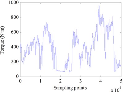
The collected data includes generator speed $n$, generator torque $T$. The training and testing processes are conducted with speed fluctuations around 3800 rpm as the dependent variable. The input features, including generator speed $n$, generator torque $T$, multi-scale torque variations $\mathrm{\Delta }T/\mathrm{\Delta }t$ over time, and speed fluctuations $\mathrm{\Delta }n$, were standardized during preprocessing to maintain a uniform scale. This standardization process could enhance model stability and minimized the risk of scale differences among features negatively impacting training outcomes. The data collected from the vehicle's bus on Dataset1 was selected as the test dataset, with data points from 50001 to 140000, as shown in Fig. 1 and Fig. 2. The data collected from the vehicle’s bus on Dataset2 was selected as the test dataset, with data points from 40001 to 90000 chosen for testing, as shown in Fig. 3 to Fig. 4.

Fig. 1Generator speed

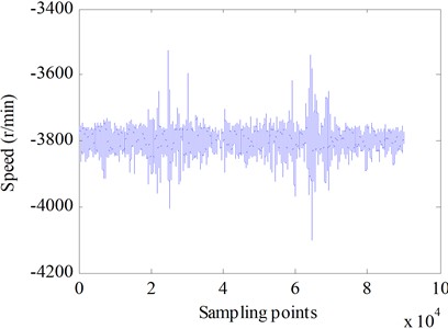
Fig. 2Generator torque

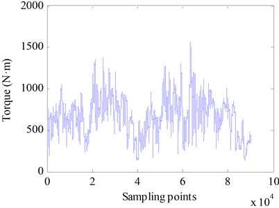
Fig. 3Generator speed

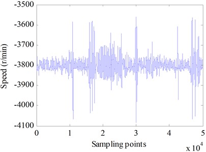
Fig. 4Generator torque

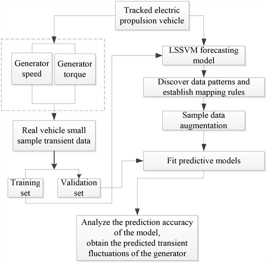
The LSSVM model’s output aligns closely with the real-time transient fluctuations of the generator under actual operating conditions. By expanding the original small sample into a larger training dataset, the model can predict future transient fluctuations of the generator, as illustrated in Fig. 5. The prediction accuracy of the LSSVM model for speed fluctuations is highly dependent on the choice of kernel function parameters. In this case, a Gaussian kernel function is selected, with optimization performed on two key parameters: the penalty factor $\gamma$ and the kernel width $\sigma$ [21, 22]. The LSSVM model uses a 10 % cross-validation method on the training sample to determine optimal parameters. This involves a two-step optimization process. First, a coupled simulated annealing algorithm is employed for coarse parameter estimation. Then, the simplex method is applied for fine-tuning and precise parameter estimation.

Fig. 5Diagram of the generator transient fluctuation prediction model

3. Real-time load prediction and control of a generator test bench

By collecting and processing real-world data from the generator in specialized electromechanical hybrid transmission systems for vehicles, the generator’s speed, torque, and rate of torque change over time are utilized as feature vectors. The machine learning algorithm LSSVM is then applied to predict the generator’s speed fluctuations in the subsequent moment, leading to the development of a test bench loading model that simulates actual vehicle generator behavior.

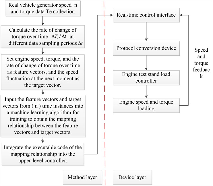
During the training process of the LSSVM, multi-scale data processing techniques are applied to the real vehicle data. This approach enhances the ability of the predicted speed to more accurately track torque variations in the test bench loading device, while also improves the model’s capacity to predict speed fluctuations within the electromechanical hybrid transmission system’s test bench. The flowchart of the generator test bench loading device and method is illustrated in Fig. 6.

3.1. Extraction of real vehicle data characteristics for electromechanical composite transmission system generators

Obtain experimental data at time $t$ by placing sensors on the actual vehicle, including the generator speed $n$ and the generator torque $T_e$, as well as the torque rate of change $\mathrm{\Delta }{T}_e/\mathrm{\Delta }t$. The calculation formula for $\mathrm{\Delta }{T}_e/\mathrm{\Delta }t$ is as follows:

10

$\frac{\mathrm{\Delta }{T}_e}{\mathrm{\Delta }t}=\frac{T_{e,t}-T_{e,t-1}}{\mathrm{\Delta }t},$

where $\mathrm{\Delta }t$ is the data sampling period, forming the feature vector $[n,T_e,\mathrm{\Delta }{T}_e/\mathrm{\Delta }t]$. Simultaneously, obtain the speed fluctuation rate $\mathrm{\Delta }n$ at time $t+1$, which represents the amplitude of fluctuation around the generator speed command issued by the electromechanical composite transmission system’s integrated controller. When there are $n$ time instances, the feature vector $[n,T_e,\mathrm{\Delta }{T}_e/\mathrm{\Delta }t]$ forms an $n\times 3$ dimensional feature matrix, while the speed fluctuation rate $\mathrm{\Delta }n$ forms an $n\times 1$ dimensional target matrix.

Fig. 6Generator test rig loading device and method flowchart

3.3. Implementation of generator loading control for electromechanical composite transmission systems

Based on the mapping relationship obtained in step (2), executable code is generated and deployed in a real-time control interface. The input data for this real-time control interface includes the current speed $n$ and the corresponding torque $T_e$ from the test rig’s generator feedback, as well as the rate of change of torque $\mathrm{\Delta }{T}_e/\mathrm{\Delta }t$ computed by the internal executable code. These three values are combined into a feature vector $[n,T_e,\mathrm{\Delta }{T}_e/\mathrm{\Delta }t]$), which is then fed into the machine learning algorithm trained in Section 3.2 to predict the next moment’s speed fluctuation value $\mathrm{\Delta }n$, as shown in Fig. 7.

Fig. 7Generator test rig loading control

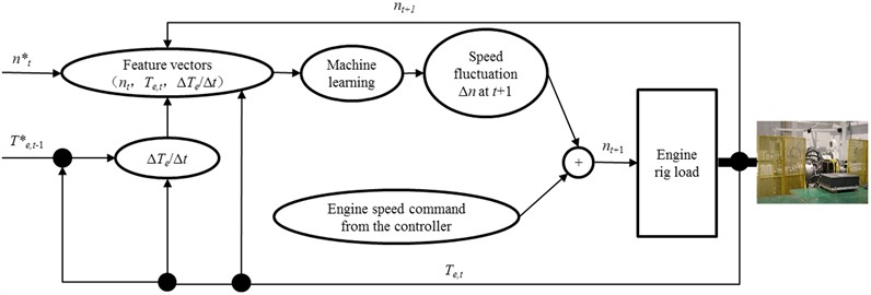
Fig. 8Prediction of engine speed fluctuations at different time scales

a) 250 ms

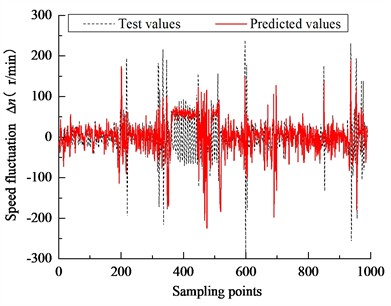
b) 500 ms

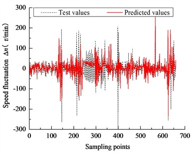
c) 750 ms

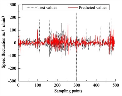
d) 1000 ms

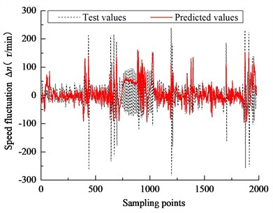
Due to the relatively small proportion of transient speed samples in the overall dataset, there is a risk of sample imbalance during machine learning training, which can lead to inaccurate predictions. To address this, it is essential to ensure that the sample sizes $\mathrm{\Delta }\mathrm{t}$ in the training and testing sets are well-matched. Taking into account the communication rate of the test rig control hardware, different data sampling intervals of 250 ms, 500 ms, 750 ms, and 1000 ms were chosen for the feature sets shown in Fig. 2 to Fig. 5 to enhance the dataset through multi-scale sampling. The parameter estimates for the LSSVM model at each scale are detailed in Table 1.

Based on the calculation process illustrated in Fig. 7, real-time engine speed feedback is replaced with LSSVM-predicted values, while torque values are derived from actual vehicle data. The initial speed is input, and the process is looped continuously to simulate the loading process. The results, as shown in Fig. 8, indicate that at sampling intervals of 250 ms, 500 ms, and 750 ms, the tracking performance between the experimental and predicted values deteriorates, with errors increasing in the middle segment of the sampling points. This degradation is primarily attributed to the time lag between response speed and change in speed. Conversely, the 1000 ms sampling interval exhibits better tracking performance with reduced error.

Table 1LSSVM parameter estimates and fitting RMSE for each time scale

Time scale	250	500	750	1000
Initial speed	–3828	–3823	–3830	–3830
$\gamma$	12.24	12.27	11.66	2.38
${\sigma }^2$	57230.5	8379.3	14982.1	2365.6
RMSE	45.2	47.5	48.6	46.4

4. Model adaptability testing under different operating conditions

The electric-driven tracked vehicle test bench is capable of reproducing the driving loads encountered by the vehicle on real road surfaces, including both resistive and inertial loads. Therefore, the load simulation platform is a critical component of the comprehensive performance test bench for electric-driven tracked vehicles. The dynamic load simulation capability is a key feature of the load simulation platform. To address this, a load simulation platform testing system has been established. The validation platform utilized in this study is an electric-drive tracked vehicle test bench, which integrates a hardware-in-the-loop (HIL) simulation platform to assess the transient speed fluctuations of the generator. The platform is comprised of five main components: the control system, driving control system, dynamic real-time simulation system, data acquisition, and monitoring system. The control system orchestrates the operation of the test bench by coordinating its control functions through the vehicle’s real-time control bus.

From the perspective of control methodology, the study integrates LSSVM-based predictive control with generator PI regulation. LSSVM predictive control is utilized to forecast fluctuations in engine speed, while generator PI control is employed to regulate torque output. Torque output, as the primary driver of engine speed fluctuations, serves as the input for engine speed dynamics. The stability of generator PI regulation is critical, as it directly impacts the amplitude of engine speed fluctuations. By coordinating these two approaches, the stability and performance of the overall system are ensured.

To enhance generalization capabilities, two primary strategies are employed. First, the diversity and comprehensiveness of the training data are significantly improved. Data is collected from a variety of driving environments and climatic conditions, encompassing a wide range of road surfaces such as cement roads, hard soil roads, muddy roads, and high-altitude terrains. This ensures that the model is exposed to diverse scenarios during the training process, enhancing its robustness and adaptability. Second, a pre-trained model is utilized to simulate the generator's standalone operation mode. By designing specific current ramps and injecting current, the model effectively simulates scenarios involving sudden load increases and decreases. This approach enables the system to better handle dynamic and complex situations, further improving its overall performance. Furthermore, the post-powertrain section of the platform controls load spikes and drops, while monitoring how the engine-generator unit in the pre-powertrain system anticipates fluctuations in engine speed due to load changes and predicts the corresponding power demands. The tests are carried out using a power motor to emulate the engine, as illustrated in Fig. 9.

Before conducting tests for the two modes mentioned above, a model tracking test was performed using real vehicle test data to validate the model’s predictive capabilities and speed tracking accuracy. The generator speed response is shown in Fig. 10 when the speed command generated by the model is applied to the test bench using actual vehicle data.

To observe the speed change trends more clearly, data processing was performed on both the speed command and the speed feedback. Specifically, an additional 50 r/min was added to the real vehicle's generator speed values, while 50 r/min was subtracted from the speed commands output by the model. From Fig. 10, it can be seen that under steady-state conditions, the generator speed fluctuations of the real vehicle remain relatively stable. However, in comparison to the model's speed command output and the generator speed feedback, the real vehicle's generator speed is more sensitive to fluctuations. The speed command generated by the model exhibits greater sensitivity when compared to the actual speed feedback.

Fig. 9Test bench verification plan

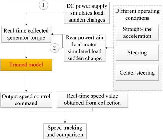
Fig. 10Real vehicle test data is used as the test set to validate the generator speed fluctuation tracking curve

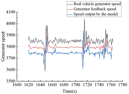
In terms of transient fluctuations, the real vehicle’s generator speed fluctuates between 3550 r/min and 4000 r/min, the model’s speed output fluctuates between 3650 r/min and 4000 r/min, and the generator speed feedback fluctuates between 3650 r/min and 3900 r/min. This indicates an error in the generator speed command output by the model, which is attributed to the model's training accuracy. Additionally, there is a discrepancy between the feedback speed value and the generator speed command, caused by the desynchronization between the command issuance cycle and the response time. The command changes occur faster than the system’s speed response capability, affecting tracking performance. This issue could potentially be addressed by adjusting the model's execution cycle. However, due to the hardware limitations of the test bench, there is a bottleneck in achieving significant improvement. Enhancements are needed in the processing capability of the main controller chip and in reducing the latency between command execution and system response. For example, utilizing a bus with higher real-time performance for data transmission and improving hardware control processing capabilities, or shortening software execution cycles, could help mitigate this issue.

Overall, based on the generator speed fluctuations observed during both steady-state and dynamic operations, and the trends of generator speed commands and feedback, the real vehicle’s fluctuations align reasonably well with the provided commands. In engineering applications, whether the model can accurately simulate generator speed fluctuations will need further validation through test bench experiments.

4.1. Generator standalone mode operation

To verify the consistency between the model’s output engine speed commands and the generator's feedback speed, an analysis of speed fluctuations was conducted under standalone operation and load step change conditions using a test stand. The generator was operated independently with a DC power source as the load, running at 3800 rpm and a high voltage of 900 V. By setting a specific load ramp, load step changes were simulated to observe the resulting speed fluctuations of the generator. Simulations were carried out under the following scenarios:

(1) Load 50 A, 100 A/s ramp to 100 A, power change rate 90 kW/s.

(2) Load 100 A, 100 A/s ramp to 200 A, power change rate 90 kW/s.

(3) Load 200 A, 100 A/s ramp to 100 A, power change rate 90 kW/s.

(4) Load 100 A, 200 A/s ramp to 300 A, power change rate 180 kW/s.

(5) Load 300 A, 200 A/s ramp to 100 A, power change rate 180 kW/s.

(6) Load 100 A, 200 A/s ramp to 300 A, power change rate 180 kW/s.

(7) Load 300 A, 100 A/s ramp to 400 A, power change rate 90 kW/s.

(8) Load 400 A, 100 A/s ramp to 300 A, power change rate 90 kW/s.

(9) Load 300 A, 200 A/s ramp to 100 A, power change rate 180 kW/s.

(10) Load 100 A, 200 A/s ramp to 500 A, power change rate 180 kW/s.

(11) Load 500 A, 200 A/s ramp to 100 A, power change rate 180 kW/s.

(12) Load 100 A, 100 A/s ramp to 50 A, power change rate 90 kW/s.

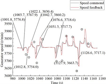
The speed curve of the generator is depicted in Fig. 11. In Fig. 11, the power rate changes for points (1), (2), (3), (4), (5), and (12) are identical, but the speed fluctuations differ. As the target current increases, the speed fluctuations become more pronounced. It can be observed that the rising slope and current change at (1) are consistent with the falling slope and current change at (12); (12) represents the reverse process of (1) and manifests as a speed increase on the waveform. Similarly, (2) and (3), as well as (10) and (11), represent opposite processes, though (10) exhibits a steeper slope and a higher target current value compared to (2).

From (1) and (2), it can be concluded that when the current change value $\nabla A$ is 50, the speed change value $\nabla R$ is 15; when the current change value $\nabla A$ is 100, the speed change value $\nabla A$ is 35; when the current change value $\nabla A$ is 200, the speed change value $\nabla R$ is 55; and when the current change value $\nabla A$ is 400, the speed change value $\nabla R$ is 90. This suggests that the current amplitude change is approximately linearly related to the speed fluctuation amplitude.

Further analysis shows that sudden changes in current (which correspond to generator torque) impact the speed fluctuations. The slope of a sudden rise or fall and the magnitude of the current are positively correlated with the slope and amplitude of the speed waveform. The sharper and larger the current change, the steeper and higher the corresponding speed waveform.

From the comparison of (4), (5), and (6), it can be deduced that sudden rises and falls in current with the same slope and amplitude do not affect the waveform characteristics; the amplitude and slope of the speed fluctuation waveform remain largely unchanged.

Additionally, it is observed that the feedback speed amplitude is magnified relative to the commanded speed amplitude, with amplification errors ranging from 0.24 % to 1.45 %. This amplification error increases with larger current changes and steeper slopes. Adjustments to the PI control system parameters can reduce this error.

Based on the above analysis, the following conclusions can be drawn: A well-calibrated model can predict generator speed fluctuations in advance and make the necessary adjustments. The generator's speed fluctuations vary with sudden load changes, and the degree of fluctuation is positively correlated with the magnitude of the load change and the steepness of the current rise or fall.

Fig. 11Generator speed curve chart

4.2. Operation mode of power chain coordination

To verify the consistency between the generator’s speed command output and the generator’s feedback speed, a front and rear powertrain coordination method is employed. This approach involves simulating load changes in the rear powertrain and observing the resulting speed fluctuations in the front powertrain. The model’s generalization capability is evaluated by validating its performance under various operating conditions based on the powertrain speed command output. Additionally, the ability of the generator controller to stabilize voltage is assessed. The generator is operated at 3800 rpm, and three distinct test conditions are considered:

– Test Condition 1: Acceleration from 0 to 32 km/h. The output speed on both sides of the transmission begins at 50 rpm and increases incrementally by 50 rpm, reaching up to 1050 rpm. The left and right drive motors each produce a torque of 230 N·m, with the target torque increased to 700 N·m at a power change rate of 100 kW/s.

– Test Condition 2: Transition between straight driving and steering. The A-side drive motor of the transmission operates at 1958 rpm, while the B-side drive motor runs at 4160 rpm. To simulate significant load disturbances with a power change rate of 100 kW/s, the torque step is set at 550 N·m/s. A load of -3042 N·m is applied to the A-side output, and a load of 6138 N·m is applied to the B-side output.

– Test Condition 3: Center steering test. The A-side output speed of the transmission is set to –172 rpm, while the B-side output speed is set to 172 rpm. Both drive motors are subjected to a torque of 50 N·m. To simulate large load disturbances with a power change rate of 100 kW/s, the torque step is set to 200 N·m/s, and a load of 500 N·m is applied. These test conditions provide a comprehensive framework to analyze the system’s performance in maintaining speed consistency and voltage stability under various dynamic load scenarios.

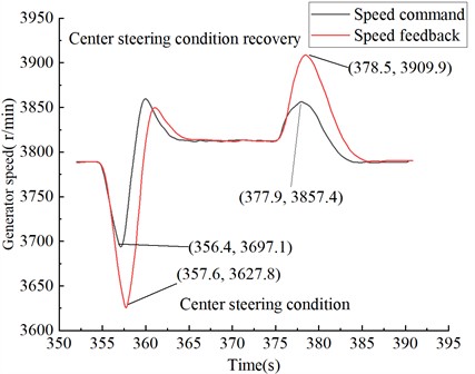
Through calculations, it has been determined that the speed command and speed response error is 1.4 % under acceleration conditions, and 1.38 % under acceleration recovery conditions, as shown in Fig. 12; 1.2 % under straight-line steering conditions, and 1.45 % under straight-line steering recovery conditions, as shown in Fig. 13; 1.9 % under center steering conditions, and 1.35 % under center steering recovery conditions, as shown in Fig. 14. These results indicate that the speed fluctuation under center steering conditions is relatively higher compared to other conditions.

Fig. 12Generator speed curve under acceleration condition during continuous driving test

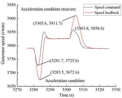
Fig. 13Generator speed curve under straight-line steering condition in Test Condition 2

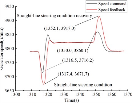
Fig. 14Generator speed curve under center steering condition in Test Condition 3

Calculate the corresponding voltage fluctuation value:

11

$U_b=\frac{\left|U_{\mathrm{m}\mathrm{a}\mathrm{x}}-U_0\right|}{U_0}\times 100\%.$

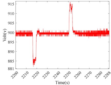
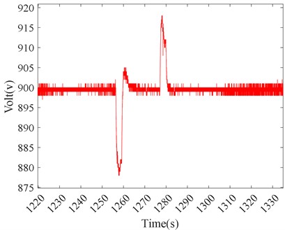
The maximum voltage fluctuation is observed to be 1.7 % under Test Condition 1, as shown in Fig. 15; 2.0 % under Test Condition 2, as shown in Fig. 16; 2.4 % under Test Condition 3, as shown in Fig. 17. All voltage fluctuations are controlled within 5 %, although a voltage fluctuation close to 5 % is seen in the actual vehicle. It can be concluded that while a larger voltage fluctuation occurs under center steering conditions compared to other conditions, the performance is still superior to the voltage fluctuations observed in the actual vehicle.

Fig. 15Generator voltage fluctuation curve under continuous driving acceleration condition in Test Condition 1

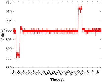
Fig. 16Generator voltage fluctuation curve under straight-line steering condition in Test Condition 2

A further analysis of the reasons for the greater speed and voltage fluctuations under center steering conditions, compared to other conditions, considering the structural characteristics of the transmission system, reveals that the transmission coefficient $i_{center}$ under center steering conditions is 17.01, while it is 3.15 under straight-line acceleration. The drive motor torque $T_{center}$ is amplified by the transmission coefficient, resulting in an output shaft torque of 8505 N·m under center steering, compared to 2205 N·m under straight-line acceleration, $T_{turnA}$ is –3042 N·m under general steering, and $T_{turnB}$ is 6138 N·m under straight-line steering. The increase in target torque for center steering leads to an increase in target current, which in turn causes larger speed and voltage fluctuations. From acceleration to straight-line steering to center steering conditions, the rising target current directly correlates with larger speed and voltage fluctuations, consistent with the analysis of generator single-unit operation.

In conclusion, the power motor experiences more severe fluctuations under center steering conditions. During center steering, speed fluctuation ranges from approximately 3600 to 3850 r/min, and during center steering recovery, it reaches 3800 to 3930 r/min. Similarly, the amplitude of voltage fluctuation increases compared to other conditions. Therefore, during actual vehicle operation, appropriate measures should be implemented under center steering conditions to prevent excessive voltage fluctuation from causing motor over-voltage issues.

Fig. 17Generator voltage fluctuation curve under center steering condition in Test Condition 3

5. Conclusions

This paper focuses on the study of mechatronic hybrid drive systems. By integrating real vehicle test data, it proposes and establishes a transient fluctuation prediction model based on the LSSVM prediction algorithm. The research involves comparing simulation values with real vehicle test data, analyzing the adaptability of the real vehicle model for fluctuation predictions, and verifying the model’s effectiveness and generalization capabilities using a mechatronic hybrid drive system test bench. The key conclusions are as follows:

1) Through the LSSVM prediction model training approach, a parameter optimization model using Gaussian functions as the space mapping mechanism is developed, aimed at optimizing penalty functions and kernel function widths. This approach effectively enhances the predictive capability of the model by comparing simulation values with real vehicle test results.

2) Using real vehicle test data as the test set, a prediction control model based on real vehicle data is established to predict control and track generator speed fluctuations. Applying predictive control to the system significantly improves both the model’s prediction accuracy and its speed-tracking performance.

3) Based on the mechatronic hybrid drive system test platform, various current ramp scenarios, target loads, and power change rates were designed for generator single-unit operating states. Through comparative analysis, speed fluctuation amplitudes and real-time performance were validated. For the front-and-rear powertrain adjustment mode, tests were designed for acceleration from 0 to 32 km/h, transitions between straight-line and steering conditions, and center steering conditions. Comparative analysis of these three scenarios and the generator single-unit operating mode showed that, under multiple operating conditions and load disturbances, the system exhibits fast dynamic recovery times, with voltage peak fluctuations within a range of ≤5 %, meeting engineering application requirements. This further validates the model's adaptability and generalization capabilities.

The results demonstrate that the LSSVM-based transient fluctuation prediction model for engine-generator sets in mechatronic hybrid drive systems provides accurate foresight for predicting engine speed fluctuations. It significantly enhances multi-power source coordination control and improves control effects related to engine speed fluctuations, offering valuable insights for engineering applications, particularly in scenarios involving traditional model predictive control approaches.