Abstract
We present a model for optimizing laser-cutting process parameters to improve fabric-cutting quality in the textile industry. We use two methods to predict fabric-cutting quality based on customized laser-cutting parameters, Response Surface Methodology (RSM) and Artificial Neural Network (ANN). RSM had an R-squared () value of 0.952, showing high accuracy. As a result of varying iterations and nodes, the results of the ANN models were different. As a result of 10,000 iterations on an architecture with six nodes and one hidden layer, the ANN model with an R-squared of 0.998 was the best optimization model. The novelty of this study found that ANNs with six nodes and 10,000 iterations optimize the laser cutting process for fabrics more effectively than models with fewer nodes and fewer iterations. RSM and ANNs are effective tools for improving fabric-cutting quality in specific applications, as well as providing theoretical contributions through this research.
1. Introduction
The fabric-cutting process in the Textile and Textile Products (TPT) industry holds significant importance and cannot be overlooked [1-3]. This process is crucial as it directly influences the final quality of the product and the profitability of the company. The precision and quality of fabric cutting have a direct impact on the final output of textile products, while the efficiency of the cutting process affects the overall production costs, thereby influencing the company’s profitability [4]. Consequently, the demand for high-quality fabric cutting has spurred advancements in the process, utilizing state-of-the-art technology to achieve optimized fabric-cutting outcomes. Laser cutting has emerged as a prominent technique in the textile industry for fabric cutting [5]. This method ensures high precision and efficiency, thereby enhancing product quality and reducing overall production costs [5]. Laser cutting quality is predominantly influenced by two machine parameters – speed and power – and one material variable, fabric thickness. The interplay of these three factors critically determines the overall cutting quality [5-7]. These parameters must be meticulously adjusted to achieve optimal cutting outcomes. Presently, the adjustment of these parameters is conducted manually, often relying on a trial-and-error approach to ascertain the most effective combination for each specific cutting task. However, the manual adjustment of these parameters is time-consuming and often results in suboptimal fabric-cutting processes using laser technology [8]. Therefore, developing a mathematical model to standardize the settings of laser cutting parameters is imperative. This approach aims to enhance the efficiency of the cutting process and ensure the production of fabric pieces of the highest quality. Artificial Neural Networks (ANNs) and Response Surface Methodology (RSM) are two prominent mathematical approaches widely employed to model parameter responses across various disciplines, including science and engineering. Artificial Neural Networks (ANNs) are computational models inspired by the structure and functioning of biological neural networks in humans. These models are adept at recognizing intricate and abstract patterns [9], [10]. In contrast, Response Surface Methodology (RSM) comprises a collection of statistical techniques used for modeling and analyzing the responses of complex systems within experimental settings. RSM aids in exploring the relationships between independent variables and system responses and optimizing these responses [11], [12]. Both approaches offer distinct advantages and disadvantages, depending on the specific requirements and nature of the problem under consideration. In some cases, integrating these methodologies can lead to optimal results [13-15]. This study employs Artificial Neural Networks (ANNs) and Response Surface Methodology (RSM) to develop models aimed at optimizing laser-cutting parameters to achieve superior fabric-cutting quality and enhanced production efficiency. The application of ANNs and RSM in this research represents a novel contribution to the field. Notably, this study is the first to formulate a model for fine-tuning laser-cutting process parameters, which are crucial in determining the quality and efficiency of fabric-cutting outcomes. The findings of this research have significant implications for the Textile and Textile Products (TPT) industry, enhancing the reliability of the production process. The developed model enables the optimal adjustment of laser-cutting process parameters, thereby ensuring the production of high-quality fabric pieces. Additionally, the model reduces the time required to fine-tune these parameters, which is traditionally a time-consuming process. Consequently, improving the efficiency and effectiveness of the laser cutting process substantially contributes to elevating the overall quality of product manufacturing within the TPT industry.
2. Research and method
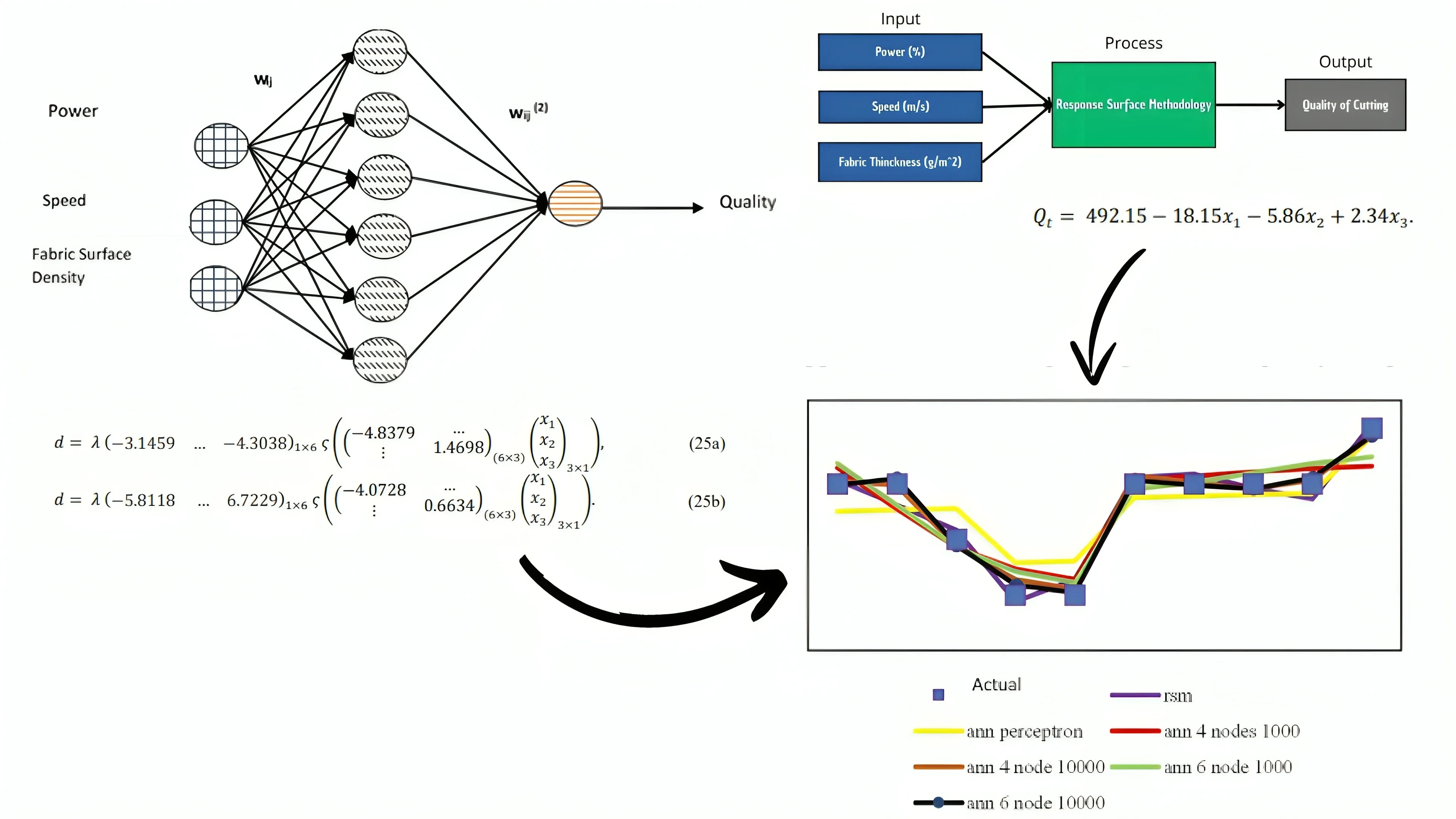
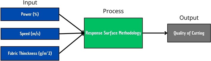
Fig. 1 illustrates the research design, which encompasses four stages: (1) data collection, (2) data preparation, (3) model development, and (4) evaluation of the model results pertaining to the tuning of laser cutting process parameters and their impact on the quality of fabric cuttings.
Fig. 1Research design
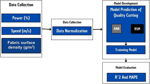
The study employs three key laser cutting process parameters: power (%), speed (m/s), and fabric surface density (g/m2), to evaluate the quality of fabric cuttings. Power indicates the percentage of power used during the cutting process, speed refers to the velocity of the laser cutting movement measured in meters per second, and fabric surface density represents the weight of the fabric per unit area. These parameters are considered independent variables that influence the quality of the fabric cut, which serves as the dependent variable. Table 1 details the specifications of the variables used in developing the fabric cut quality prediction model.
Table 1Specification model
Parameter | Unit | Function |
Quality of cutting | Index | Dependent variable |
Power | % | Independent variable |
Speed | m/s | |
Fabric surface density | g/m2 |
3. Result and discussion
3.1. Data collection
The experimental data from the Textile and Textile Products (TPT) industry were meticulously gathered by experts adhering to the industry-specific standards. Table 2 shows the three process parameters as the independent variables, with piece quality serving as the dependent variable.
Table 2Data collection
Sample | Input | Output | ||
(Power (%)) | (Speed (m/s)) | (Fabric surface density (g/m2)) | (Quality) | |
1 | 26 | 98 | 238.5 | 3 (Moderate Quality) |
2 | 26 | 103 | 250.8 | 3 (Moderate Quality) |
3 | 26 | 108 | 263.2 | 2 (Good Quality) |
4 | 26 | 113 | 275.5 | 1 (Excellent quality) |
5 | 26 | 118 | 287.9 | 1 (Excellent quality) |
6 | 31 | 98 | 277.9 | 3 (Moderate Quality) |
7 | 31 | 103 | 290.2 | 3 (Moderate Quality) |
8 | 31 | 108 | 302.5 | 3 (Moderate Quality) |
9 | 31 | 113 | 314.9 | 3 (Moderate Quality) |
10 | 31 | 118 | 327.3 | 4 (Poor Quality) |
Table 3Data normalization
(Power (%)) | (Speed (m/s)) | (Fabric surface density (g/m2)) | (Quality) |
0 | 0 | 0 | 0.666666667 |
0 | 0.25 | 0.139065614 | 0.666666667 |
0 | 0.5 | 0.278131228 | 0.333333333 |
0 | 0.75 | 0.417196843 | 0 |
0 | 1 | 0.556262457 | 0 |
1 | 0 | 0.443658721 | 0.666666667 |
1 | 0.25 | 0.582724335 | 0.666666667 |
1 | 0.5 | 0.721789949 | 0.666666667 |
1 | 0.75 | 0.860855563 | 0.666666667 |
1 | 1 | 0.999921177 | 1 |
3.2. Data preparation
To prepare data for Artificial Neural Network (ANN) modeling, standardization and normalization are essential procedures to ensure data uniformity. Beyond aiding the ANN training process, normalization can improve the model’s convergence. In this study, normalization is conducted using the method, as in Eq. (1):
where represents the normalized data, where is the smallest value in the dataset, and is the highest value in the dataset. Table 3 shows the results of the data normalization.
3.3. development
3.3.1. ANN model for quality of cutting
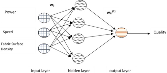
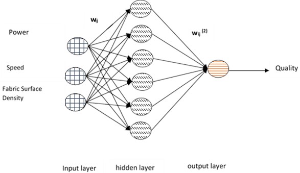
The ANN model has three input neurons, which indicate power, speed, and fabric surface density. The output layer determines laser cutting quality. Eqs. (2) and (3) can be used to express the hidden layer output ( ) as well as the quality of the laser cutting result ():
where represents the value of the hidden layer neuron, denotes the input neuron, is the bias, signifies the weight from the input to the hidden layer, is the activation function, and in this study, a sigmoid activation function is employed represents the weight of the output neuron. In this research, ANN architecture was created that incorporates three types of nodes into a single hidden layer. These variants were used to determine the best model, which was defined by minimal evaluation criteria. Fig. 2 shows the structure of the Perceptron used in this first model.
Fig. 2Neural network architecture model of perceptron
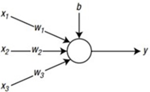
3.3.1.1. Perceptron model
The model employed consists of three input neurons and one output neuron, as illustrated in Fig. 2. The determination of weights, as referenced in Eq. (2), can be derived through Eqs. (4) to (6):
Then, in matrix form, the sum of the weights () can be expressed in equations follows:
A simple one-node model can be stated as follows, where is the node’s index and is the index of the input . In a one-node output model with three inputs, the bias can be ignored as it is a factor related to information storage and acquired as a constant in the model. To calculate this result, we use the activation function in Eq. (10):
3.3.1.2. The feed forward ANNs with four nodes in one hidden layer
In the second ANN model architecture, a feed-forward propagation model was constructed, comprising four nodes within a single hidden layer. This architecture was evaluated under two different iteration scenarios: the first with 1,000 iterations and the second with 10,000 iterations. The effectiveness of both models was assessed using the correlation coefficient and mean absolute percentage error (MAPE). Fig. 3 depicts the architecture of this ANN model.
Fig. 3Architecture ANNs with four node one hidden layer
In Fig. 3, the arrows and circles represent the signal flow and neurons, respectively. The weight matrices of the first and second layers are denoted by the terms () and (). The weighted sum can be determined using Eqs. (10) and (11):
The terms and are the weighted sum of the first layer and the first layer weight matrix, respectively. The terms , , and are the input parameters. The neuron feeds the weighted sum into the sigmoid function and produces the result shown in Eq. (12):
Eq. (12) is the input of the second layer, which results in a weighted sum, , at the second layer, as seen in Eqs. (13) and (14):
The neuron inputs the weighted sum into a linear function, which generates the output. The neuron’s properties is characterized by this linear output function, as expressed in Eqs. (15) and (16):
The constants derived through the optimization process in Eqs. (15), (16a) and (16b), as well as the ANN architecture with four nodes in one hidden layer for 1,000 and 10,000 iterations, are detailed in Eq. (17a) and (17b):
3.3.1.3. Feed-forward ANNs with a sixth node in one hidden layer
In the third ANN model architecture, a feed-forward propagation model was developed, comprising six nodes within a single hidden layer. This architecture was subsequently tested with two different iteration scenarios: the first with 1,000 iterations and the second with 10,000 iterations. The effectiveness of both models under these iteration variations was then assessed using the correlation coefficient and Mean Absolute Percentage Error (MAPE) metrics. Fig. 4 illustrates the architecture of this ANN model.
Fig. 4Architecture ANNs with sixth node one hidden layer
In Fig. 4, the arrows and circles represent the signal flow and neurons, respectively. The weight matrices of the first and second layers are denoted by the terms () and (). The weighted sum can be determined using Eqs. (18) and (19):
The terms and are the weighted sum of the first layer and the first layer weight matrix, respectively. The terms , , and are the input parameters. The neuron feeds the weighted sum into the sigmoid function and produces the result shown in Eq. (20):
Eq. (20) is the input of the second layer, which results in a weighted sum, , at the second layer, as seen in Eqs. (21) and (22):
The neuron passes the weighted sum to a linear function, which generates the output. The linear output function, as given in Eqs. (23) and (24), identifies the neurons function:
The constants derived through the optimization process in Eqs. (23), (24a) and (24b), as well as the ANN architecture with four nodes in one hidden layer for 1,000 and 10,000 iterations, are detailed in Eq. (25a) and (25b):
The result of the mapping is measured based on three different ANN models, with different nodes in the hidden layer, and different iterations for each model. Table 4 shows the optimized results for the ANNs architecture model.
Table 4Result of ANNs model
Actual | Perceptron model | One hidden layer (4 nodes) | One hidden layer, (6 nodes) | ||
Iteration 1,000 | Iteration 10,000 | Iteration 1,000 | Iteration 10,000 | ||
3 | 2.5 | 3.2836 | 3.0694 | 3.3619 | 2.9725 |
3 | 2.527 | 2.5426 | 2.9647 | 2.6119 | 3.0922 |
2 | 2.5537 | 1.855 | 1.8676 | 1.8586 | 1.8928 |
1 | 1.5807 | 1.4635 | 1.2769 | 1.4203 | 1.1776 |
1 | 1.6074 | 1.279 | 1.1026 | 1.2223 | 1.0375 |
3 | 2.7496 | 3.0604 | 3.1558 | 2.9011 | 3.0565 |
3 | 2.7757 | 3.1381 | 3.025 | 3.0214 | 2.9716 |
3 | 2.8015 | 3.2122 | 2.9053 | 3.1927 | 2.9074 |
3 | 2.8273 | 3.2734 | 3.064 | 3.3598 | 3.1069 |
4 | 3.8528 | 3.3169 | 3.85 | 3.481 | 3.8608 |
3.3.2. RSM model for quality of cutting
In this investigation, the RSM model is constructed based on three independent variables: Power (), speed (), and fabric surface density (), which collectively influence the Quality of Fabric Cutting (). The core equation of RSM is represented as follows Eq. (26):
where, , , and denote the independent variables, specifically power, speed, and fabric surface density, respectively. The terms , , , and represent the regression model constants for the respective variables, while ε represents the model error. Fig 5 illustrates the architecture of the RSM model used.
Fig. 5RSM architecture model
To obtain the constant value of Eq. (26), it can be determined by modeling it as illustrated in Eqs. (27) and (28):
The difference between the experimental data, and the model is defined as the error , which is as follows:
Using Eqs. (29) and (30), we use to find the model:
Eq. (14) can be used to solve the linear equation produced by Eq. (26), resulting in the formulation shown in Eqs. (31) to (34):
Eq. (31) can be converted into matrix form as in Eq. (32):
The values of , , in Eq. (31) are obtained through the parameter optimization method, as in Eq. (33):
Then, Eq. (34) is derived to assess the quality of fabric cutting results using laser cutting, as follows:
In Table 5, Eq. (34) is used to calculate prediction calculations to assess the quality of fabric cutting after , , , and have been determined.
Table 5RSM model prediction results
(Quality of fabric cutting) prediction | (Quality of fabric cutting) actual |
30651 | 3 |
26168 | 3 |
21685 | 2 |
08778 | 1 |
12719 | 1 |
31137 | 3 |
31729 | 3 |
29192 | 3 |
27246 | 3 |
40695 | 4 |
3.4. Evaluation result model
3.4.1. MAPE (mean absolute percentage error)
A model's performance can be evaluated using the Mean Absolute Percentage Error (MAPE). Most commonly, it is used to determine the accuracy of predictive models, particularly in numerical or time series prediction. MAPE is calculated by comparing the actual and predicted values of a model. Eq. (35) demonstrates the calculation of MAPE:
MAPE is presented as the difference between the absolute amount predicted by the model (At) and the actual amount of experimental data () divided by the actual amount of experimental data (Ft) multiplied by 100 %. Therefore, using Eq. (35), the quality of fabric cutting predicted using both Artificial Neural Networks (ANN) and Response Surface Methodology (RSM) methods can be found in Table 6 as the absolute average of predictions.
3.4.2. Coefficient of determination (R2)
The coefficient of determination, also known as R-squared or , is a statistical metric that measures how well a theoretical model matches actual observed data. In this context, indicates the quantity of variance in the dependent variable can be explained by the independent variables included in the model. The value of ranges from 0 to 1. A score of 1 shows that the model completely explains the variation in the data, whereas a value of 0 indicates that the model explains no variation and is simply a random error. Eq. (36) shows the calculations for the two model techniques developed:
The interpretation obtained from both the Artificial Neural Networks (ANNs) and Response Surface Methodology (RSM) models represents the developed model's ability to explain the complete variability in the dependent variable. Eq. (37) can be used to calculate the coefficient of determination in the prediction results for the total quantity of quality laser cutting performed with both the ANN and RSM techniques, as shown in Table 6.
This research requires neural computing because the process of laser-cutting fabric involves many complex and non-linear variables and interactions, which are difficult to model with deterministic rules or simple regression. Simple regression cannot effectively capture the complex relationships between process parameters and cutting quality, resulting in correctable prediction errors. Neural networks, with their ability to learn non-linear patterns and handle varying data, can provide more accurate and adaptive models, reducing prediction errors significantly.
Table 6Result of the evaluation model
Evaluation model | RSM | Perceptron | ANN one hidden layer (4 nodes) | ANN one hidden layer (6 nodes) | ||
Iteration 1,000 | Iteration 10,000 | Iteration 1,000 | Iteration 10,000 | |||
0.952 | 0.544 | 0.855 | 0.979 | 0.884 | 0.998 | |
MAPE (%) | 0 | 0.863 | 1.607 | 1.070 | 1.630 | 0 |
3.4.3. Analyze evaluation result
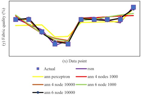
The Response Surface Methodology (RSM) and Artificial Neural Networks (ANNs) can be used to optimize laser cutting settings for better fabric cutting quality. The ANN-based model, constructed through 10,000 iterations with a six-node architecture on a single hidden layer, demonstrated superior performance, with a mean absolute percentage error (MAPE) value of 0 % and a coefficient of determination () of 0.998. This implies that the model effectively accounts for 99.8 % of the variance in the actual data on fabric-cutting quality. The architecture type and complexity of the nodes and hidden layers used have a significant impact on the variability in validation results for ANN models. The RSM model performed well in predicting laser cutting parameters for cutting quality, with a MAPE score of 0 % and a of 0.952. Nonetheless, there are differences in the explained variance by the RSM method, which could be resolved by using more complex model optimization techniques such as ANNs. The gap in the R² value of the RSM model, which remains accessible to development, emphasizes the preference for ANN-based models for deeper insights. Fig. 6 shows the dispersion of actual cutting quality data received from garment industry professionals, compared with model outcomes, to clearly highlight the optimization model's variance. Furthermore, the findings highlight the significant impact of changing process factors like as power, speed, and fabric surface density on cutting quality. These findings may aid in the development of a standardized parameter index for optimizing laser cutting parameters in textile applications, hence improving fabric cut quality and process efficiency.
Fig. 6Pattern distribution of data
4. Conclusions
In conclusion, this research has successfully developed an optimization model to assist in adjusting laser cutting process parameters that affect the quality of fabric in the textile and textile products (TPT) industry. The Response Surface Methodology (RSM) model accurately predicts fabric quality, with an of 0.95. The ANNs model with six nodes and 10,000 iterations performs well in optimizing cutting process parameters in terms of fabric cutting quality, with a lower error rate than models with fewer nodes and iterations (MAPE 0 % and value of 0.998). The examination of the optimization results shows that the ANNs RSM-based model is the most successful at predicting fabric cutting quality when laser cutting settings are adjusted. These findings have practical relevance for textile industry practitioners, particularly in the textile sector, and give an important framework for optimizing laser cutting process parameters and enhancing cutting quality in fabric markets. Furthermore, the use of Response Surface Methodology (RSM) and Artificial Neural Networks (ANNs) to model fabric quality provides a new perspective on mathematical modeling in textile manufacturing, emphasizing the utility of statistical methods like RSM in analyzing and improving manufacturing processes.
References
-
M. Tabraz, “Importance of fashion cad (computer aided design) study for garment industry in Bangladesh,” International Journal of Scientific and Technology Research, Vol. 6, No. 10, pp. 26–28, May 2024.
-
U. Bristi and M. Al-Mamun, “Productivity improvement of cutting and sewing section by implementation of value steam method in a garments industry,” American Scientific Research Journal for Engineering, Technology, and Sciences, Vol. 54, No. 1, pp. 185–202, 2019.
-
E. Enes and Kipöz, “The role of fabric usage for minimization of cut-and-sew waste within the apparel production line: Case of a summer dress,” Journal of Cleaner Production, Vol. 248, p. 119221, Mar. 2020, https://doi.org/10.1016/j.jclepro.2019.119221
-
A. P. D. M. Kayar and Y. Karatepe Mumcu, “Using neural network method to solve marker making ‘calculation of fabric lays quantities’ efficiency for optimum result in the apparel industry,” in 8th WSEAS International Conference Simulation, Modelling and Optimization, 2008.
-
R. Nayak and R. Padhye, “The use of laser in garment manufacturing: an overview,” Fashion and Textiles, Vol. 3, No. 1, Mar. 2016, https://doi.org/10.1186/s40691-016-0057-x
-
R. E. Permatasari, M. Cory, A. Siagian, and K. Kunci, “Pengaplikasian teknik laser cut sebagai embellishment pada modest wear,” eProceedings of Art and Design, Vol. 6, No. 3, pp. 4189–4197, 2019.
-
E. Yulianto, “Deteksi kondisi ambang batas dalam teknik fabrikasi laser menggunakan fotoluminesensi,” Jurnal Crankshaft, Vol. 4, No. 2, pp. 1–8, Oct. 2021, https://doi.org/10.24176/crankshaft.v4i2.6449
-
N. Yusoff, N. A. A. Osman, K. S. Othman, and H. M. Zin, “A study on laser cutting of textiles,” 29th International Congress on Laser Materials Processing, Laser Microprocessing and Nanomanufacturing, Vol. 103, pp. 1559–1566, Jan. 2010, https://doi.org/10.2351/1.5062018
-
V. G. V. Putra and J. N. Mohamad, “A novel model for predicting tenacity and unevenness of ring-spun yarn: a special case in textile engineering,” Mathematical Models in Engineering, Vol. 9, No. 3, pp. 102–112, Sep. 2023, https://doi.org/10.21595/mme.2023.23406
-
A. Mukhopadhyay, “Application of artificial neural networks in textiles,” Textile Asia, Vol. 33, No. 4, pp. 35–39, 2002.
-
S. B. Jadhav, A. S. Chougule, D. P. Shah, C. S. Pereira, and J. P. Jadhav, “Application of response surface methodology for the optimization of textile effluent biodecolorization and its toxicity perspectives using plant toxicity, plasmid nicking assays,” Clean Technologies and Environmental Policy, Vol. 17, No. 3, pp. 709–720, Aug. 2014, https://doi.org/10.1007/s10098-014-0827-3
-
K. Karthikeyan, K. Nanthakumar, K. Shanthi, and P. Lakshmanaperumalsamy, “Response surface methodology for optimization of culture conditions for dye decolorization by a fungus, aspergillus niger hm11 isolated from dye affected soil,” Iranian Journal of Microbiology, Vol. 2, No. 4, pp. 214–223, 2010.
-
M. S. Kothari, K. G. Vegad, K. A. Shah, and A. Aly Hassan, “An artificial neural network combined with response surface methodology approach for modelling and optimization of the electro-coagulation for cationic dye,” Heliyon, Vol. 8, No. 1, p. e08749, Jan. 2022, https://doi.org/10.1016/j.heliyon.2022.e08749
-
V. G. V. Putra and J. N. Mohamad, “Response surface methodology and artificial neural network modeling of work of adhesion on plasma-treated polyester-cotton-woven fabrics,” Journal of Adhesion Science and Technology, Vol. 37, No. 6, pp. 976–996, Mar. 2023, https://doi.org/10.1080/01694243.2022.2053349
-
H. Toutenburg, “Statistical analysis of designed experiments,” in Springer Texts in Statistics, New York, NY: Springer New York, 2009, https://doi.org/10.1007/978-1-4419-1148-3
About this article

The authors have not disclosed any funding.
The authors express their gratitude for the assistance provided throughout this inquiry. Special thanks are extended to colleagues who helped with data collection. Their amazing assistance and support made a huge contribution to the project’s success.
The datasets generated during and/or analyzed during the current study are available from the corresponding author on reasonable request.
Muhamad Danil Pratama and Fadil Abdullah collected the data. Fadil Abdullah and Valentinus Galih Vidia Putra worked on model development and calculations. Lisa Samura, Yusril Yusuf, Valentinus Galih Vidia Putra, Fandi Achmad, and Fadil Abdullah wrote and revised the manuscript.
The authors declare that they have no conflict of interest.
