Abstract
Regression analysis is essential for prediction analysis and variable identification since air pollution studies are complicated by competing suggestions and require careful interpretation. In the existing predictive analysis, estimating indoor radon levels is challenging due to multicollinearity issues and the existing algorithm's assumption of independent predictor variables, making it difficult to accurately assess individual effects. Hence a novel Unsupervised Bayesian Multiple Regression Analysis is used to correctly offer the specific impacts of each predictor variable by taking the complex interactions between factors in the estimation of indoor radon levels. Furthermore, in the variable identification, indoor radon levels are influenced by complex residual distributions, with existing algorithms failing to predict non-Gaussian residuals due to outlier-sensitive least squares estimation. So a novel Quadratic Discriminant Extreme Learning Machine is implemented to overcome this issue, which creates models that are better able to reliably detect the factors driving indoor radon levels and are more robust to non-Gaussian residual distributions. The proposed method demonstrates excellence in predictive analysis and variable identification achieving high coefficient of relation and low MAE.
1. Introduction
The natural decay of uranium in the earth's crust produces radon, a radioactive gas that poses health risks. Radon enters the soil, undergoes advection and diffusion, and is released into space. Environmental factors such as temperature and humidity influence its exhalation rate [1]. Dosimeter detectors provide comprehensive data on average long-term exposure levels by measuring and recording radon concentrations over 12 months. This information is essential for risk assessment, mitigation strategy implementation, and well-informed policy formulation to safeguard public health [2]. The following factors affect indoor radon concentrations: humidity, temperature, and pressure. Air circulation is impacted by temperature, radon adsorption and buildup are impacted by humidity, and entrance and departure are impacted by pressure differentials. Comprehending these associations is essential for formulating efficacious tactics and pinpointing situations with elevated danger [3].
High quantities in geogenic materials and building sealing techniques lead to radon seepage into interior spaces. Radon seepage is caused in part by soil and building air exchange rate. Enhancing ventilation, depressurizing sub-slabs, caulking access sites, and altering the soil are examples of mitigation techniques. It’s essential to regularly assess indoor air quality [4]. In Italy’s Euganean Hills, researchers analyze radon's origins and regulating factors to create hazard prediction maps. These maps guide targeted mitigation efforts, addressing the region's elevated radon levels, the second leading cause of lung cancer. Collaborative strategies and regulations aim to safeguard public health through informed awareness and preventive measures [5].
Uranium and thorium, primordial radionuclides in the earth’s crust, undergo decay processes, producing radon and thoron noble gases with potential health implications. The concentration of radon is influenced by soil radium content, radiating power, and moisture levels. Variances in these soil characteristics impact the emanation of radon, contributing to fluctuations in indoor air levels. Moreover, environmental factors, including carbon dioxide acting as a carrier gas, play a pivotal role in radon transport through soil. Understanding these intricate interactions is vital for assessing radon exposure risks and implementing effective mitigation strategies, especially in regions where geological conditions may contribute to heightened radon concentrations [6]. Radon concentrations exhibit considerable variability influenced by diverse factors, including tectonic events, geochemical origins, weather patterns, and human activities. Tectonic events, such as earthquakes or ground movements, can impact soil structures and subsequently affect radon release. Geochemical origins, encompassing the distribution of radionuclides in geological formations, significantly contribute to regional radon disparities. Weather conditions, including temperature and precipitation, influence radon transport and diffusion. Human activities, like construction and mining, can disturb radon-rich geological formations, altering its release dynamics. To navigate this complexity, machine learning techniques are proposed. These advanced algorithms can analyze vast datasets, considering temporal and geographical variables, enhancing our understanding of radon dynamics for more targeted risk assessment and mitigation strategies [7-9].
Chronic Obstructive Pulmonary Disease (COPD), a prevalent respiratory condition impacting 300 million people globally, poses significant public health challenges. Radon exposure, a known source of ionizing radiation, has been associated with DNA damage and an increased risk of lung cancer. This linkage between COPD and radon exposure was substantiated in a comprehensive 2020 study, emphasizing the potential health ramifications. The study revealed a correlation between atmospheric radon levels during dust occurrences and improved regression coefficients. This underscores the critical need for understanding the interplay between environmental factors, radon exposure, and respiratory health to devise targeted preventive measures and healthcare interventions for COPD [10-11]. Lung cancer, a leading cause of global cancer-related deaths, is primarily linked to indoor radon exposure, posing a significant public health risk. Recognizing this threat, Spain and the European Union have implemented radon protection laws since 2019 to control workplace exposure. These regulations focus on mitigating the risk of elevated radon concentrations in enclosed environments. By enforcing preventive measures, such as improved ventilation and building design, these laws aim to limit radon infiltration and protect workers from potential health hazards. The proactive approach underscores a commitment to public safety, emphasizing the importance of regulatory frameworks in minimizing the impact of indoor radon on lung cancer incidence [12]. In Montenegro, a dedicated project endeavors to forecast indoor radon concentrations surpassing the national limit, employing advanced statistical methods like logistic multivariate regression. This technique enables the project to analyze multiple variables simultaneously, including geological factors, building characteristics, and environmental conditions. By harnessing a comprehensive dataset, the project seeks to develop a predictive model that identifies areas prone to exceeding the national radon limit of 200 Bq/m3 in newly constructed buildings. The utilization of logistic multivariate regression underscores a commitment to data-driven risk assessment, allowing for targeted interventions and ensuring compliance with radon exposure standards to safeguard public health in Montenegro [13-14].
Climate change in Bulgaria brings significant variations in climatic factors, affecting radon levels. Decision trees, such as CART-type algorithms, are used to analyze predictors in radiological cave research [15-16]. Tobacco smoking is a leading modifiable risk factor for lung cancer, accounting for 32.5 % of smoking-related mortality in Spain. Radon exposure, as the second greatest contributor, is studied in relation to small cell lung cancer in the Small Cell Study [17-18]. This comprehensive overview underscores the complex interplay of environmental factors, health risks, and regulatory efforts in the context of radon.
The Major contributions in this paper are given as follows:
1) To predict the indoor radon levels, a novel Unsupervised Bayesian Multiple Regression Analysis has been introduced which enhances prediction accuracy by accounting for complex interactions between factors, allowing for a more precise estimation of the specific impacts of each predictor variable on indoor radon levels.
2) To identify variables affecting indoor radon levels, a novel Quadratic Discriminant Extreme Learning Machine (QDELM) is proposed for the enhanced resilience to non-Gaussian distributions which enables more reliable detection of the factors driving indoor radon levels, leading to more precise predictions.
The above-mentioned contributions have been taken into consideration to address the issues with the current approaches. The content of the paper is arranged as follows: The literature study is covered in Section 2, the methodology and operation of the proposed method are explained in Section 3, and the evaluation, performance analysis, and comparison elements of the proposed framework are covered in Section 4. The conclusion of the study is found in Section 5.
2. Literature survey
Shboul et al. [19] presented the eXtreme Gradient Boosting (XGBoost) and Light Gradient Boosting Machine (LightGBM) machine learning (ML) techniques, which are backed by multivariate analysis (MA). A set of soil samples were subjected to an investigation that included measurements of radon surface exhalation rates as well as relevant characteristics including moisture content, particle size distributions, and concentrations of Ra-226, Th-232, and K-40. The investigation identified a number of critical variables, including moisture content, Ra-226 concentration, and bigger soil particles, that affect radon exhalation rates. Contour plots of the experimental and machine learning produced data were made to show the complex interactions between these factors. These illustrations showed that higher soil moisture content reduces the pace at which radon is exhaled. However, there were limits to this research’s ability to identify significant adverse effects.
Seyis et al. [20] were installed in six monitoring stations in Western Turkey: four in Gebze, one in Armutlu, and one in Sarıköy. Eight distinct parameters (soil radon, soil temperature, soil moisture, air temperature, air pressure, precipitation, wind speed, and wind direction) were measured at these sites during 18 months from April 2008 to November 2010. Thus, every 15 minutes, soil radon was measured every 60 minutes, and data on soil temperature, moisture content, air temperature, air pressure, precipitation, wind direction, and speed was recorded. Eventually, correlation coefficients were found between these variables. Nevertheless, this work uses in situ measurements over a long period to evaluate temporal fluctuations in soil radon concentrations and their relationships with possible regulating factors.
Joo et al. [21] presented the association, using multiple regression analysis and huge data of those factors, between the ambient radiation dose rate and meteorological variables. On Ulleung Island, Republic of Korea, measurements were made of 36 distinct climatic variables and the rate of ambient radiation dosage between 2011 and 2015. The primary meteorological factors impacting the ambient radiation dose rate were discovered by applying stepwise selection methods and Pearson correlation analysis to the large dataset. These variables were then employed as the independent variables for the regression model. Multiple regression models were then created for the monthly datasets as well as the dataset for the full period. However, the various meteorological factors have varying degrees of effect throughout time and have a considerable impact on the rate of environmental radiation exposure at different times.
Benà et al. [22] implemented a robust multivariate machine learning technique (Random Forest) to generate the GRP map of the Pusteria Valley's core sector. The risk map was generated by combining other census tract characteristics, such as population as an exposure factor and land use as a vulnerability component. The pilot site was selected from the Pusteria Valley in northern Italy because of its well-known structural, geochemical, and geological characteristics. The findings show that residential areas and high population densities, together with high GRP values, are related to high Rn risk locations. When it builds up in small spaces, though, it becomes a major health risk.
Haider et al. [23] developed advanced methods, including decision trees (DT), multiple linear regressions (MLR), and artificial neural networks (ANN), to better and more consistently identify radon anomalies of the tectonically active origin in northern Pakistan. The soil radon concentration and related climatic factors obtained at a seismically active area in northern Pakistan comprise the dataset used in the proposed research. The recorded dataset is split using a time frame of ±7 days surrounding the time of the earthquake into seismically active (SA) and stable (NSA) phases. Using three inputs (meteorological variables) and one output parameter (radon), intelligent algorithms are trained and cross-validated on the NSA dataset. It is currently unclear how to reliably identify radon anomalies that have been caused by seismic activity.
Panahi et al. [24] introduced a novel modeling procedure to estimate the radon potential in the northwest of Gangwon Province, South Korea, utilizing deep learning models based on convolution neural network (CNN), long short-term memory (LSTM), and recurrent neural network (RNN). The data used in this study are divided into two sets: independent variables (radon conditioning factors: lithology, distance from lineament, mean soil concentrations of calcium oxide [Cao], potassium oxide [K2O], and ferric oxide [Fe2O3], effective soil depth, topsoil texture, and soil drainage) and dependent variables (measured soil gas radon concentrations). However, the scarcity of knowledge makes mapping radon potential difficult.
Zhang et al. [25] Using these variables as a basis, decision tree models were built to simulate the “background” radon fluctuation and detect anomalies by contrasting the observed radon changes with the “background” variations. With a 0.8 correlation coefficient, the predicted “background” variation and the observed data from the non-seismic activity period are well correlated. Next, the study contrasted the observed radon time series variation during the seismic activity period with the modeled "background" fluctuation. Out of the 24 selected earthquakes, the decision tree could find 15 potential radon abnormalities. The observed variations in spring flow and water temperature provide additional evidence for the highlighted abnormalities. However, a variety of interfering variables impacted the radon levels in groundwater.
Pirkkanen et al. [26] investigated the development of lake whitefish (Coregonus clupeaformis) in two distinct, one-of-a-kind laboratory settings: 2 km below the surface of the Earth and in a radiation-shielded environment 2 km below the surface. Lake whitefish embryos raised in these two facilities were compared for differences using morphometric analysis and established developmental endpoints. Regarding hatch date and survival rate, no appreciable distinctions were found between the surface and subterranean facilities. In embryos raised underground, there was a notable increase of up to 10 % in both body weight and length. However, the lack of a scientific infrastructure to support the studies limits the amount of biological study that is done in deep-underground settings.
Li et al. [27] proposed a multi-stage ensemble-based model using monthly gross beta particle radioactivity distributions with a spatial resolution of 32 km over the contiguous United States from 2001 to 2017. In the contiguous United States, 129 RadNet sensors recorded particulate radioactivity. In the first step, researchers used six strategies to build 264 base learning models, from which researchers picked nine base models with varying predictions. Using a non-negative weighted regression technique, researchers aggregated the base learner predictions of the chosen candidates in stage two, taking into account their local performance and geography. For exposure assessment, there aren’t any geographically and temporally resolved particle radioactivity data available at this time.
Njoku et al. [28] presented the 2002–2020 period's link between LULC, elevation, and LST in Ilorin. Understanding the degree of correlation between LULC, elevation, and LST as well as the factors influencing the temporal and geographical fluctuation in the connection was the main goal. Landsat data products were used to create LST and NDVI. A mono-window technique was utilized to generate LST, and the NDVI was employed as a stand-in for LULC. LULC's geographical pattern was examined by the use of Moran's I spatial autocorrelation statistics. The precise path by which recognized elements influence the thermal character of the urban environment, as well as the factors that influence the geographical and temporal fluctuation of the link between LULC and the LST, remain unclear.
From the above studies it is clear that in [19] The capacity of this study to detect notable negative effects was limited, in [20] Study employs in situ measurements to assess temporal soil radon fluctuations and correlations, in [21] Meteorological factors exhibit varying effects, influencing environmental radiation exposure rates differently over time, in [22] High radon risk linked to residential areas, dense populations, and elevated GRP values. Major health risk in confined spaces, in [23] Identifying seismic-induced radon anomalies remains unclear; reliable methods are currently elusive, in [24] The difficulty in mapping radon potential stems from a lack of understanding, in [25] The radon levels in groundwater were affected by many interacting factors, in [26] Insufficient scientific infrastructure hampers biological studies in deep-underground settings, in [27] Lack of geographically and temporally resolved particle radioactivity data hinders exposure assessment, in [28] Unclear how recognized elements impact urban thermal characteristics and LULC-LST fluctuations geographically. Hence, there is a need for a novel method to eliminate these drawbacks and improve the accuracy of variable identification and predictive analysis.
Table 1Research studies on radon and radiation analysis
Ref. No | Techniques used | Effectiveness |
[19] | XGBoost, LightGBM, multivariate analysis | Identified critical variables affecting radon exhalation rates, demonstrated complex interactions between factors |
[20] | Correlation analysis, in situ measurements | Evaluated temporal fluctuations in soil radon concentrations and their relationships with regulating factors |
[21] | Multiple regression analysis, stepwise selection methods, Pearson correlation analysis | Identified primary meteorological factors impacting ambient radiation dose rate, created regression models for monthly and full-period datasets |
[22] | Random Forest, multivariate analysis | Generated GRP map of Pusteria Valley's core sector, identified high radon risk locations |
[23] | Decision trees, multiple linear regression, artificial neural networks | Developed methods to identify radon anomalies of tectonic origin in northern Pakistan, trained algorithms on seismic and stable datasets |
[24] | Convolutional neural network, long short-term memory, recurrent neural network | Used deep learning models to estimate radon potential in Gangwon Province, South Korea |
[25] | Decision trees, correlation analysis | Built decision tree models to simulate background radon fluctuations and detect anomalies during seismic activity |
[26] | Morphometric analysis, comparison studies | Investigated development of lake whitefish embryos in underground settings, found notable differences in body weight and length |
[27] | Ensemble-based model, weighted regression | Proposed a multi-stage ensemble-based model for exposure assessment using gross beta particle radioactivity distributions |
[28] | Correlation analysis, spatial statistics | Explored link between LULC, elevation, and LST in Ilorin, identified factors influencing temporal and geographical fluctuation |
Table 1 presents various research studies on radon and radiation analysis, highlighting the effectiveness of various techniques. These studies include utilizing advanced machine learning techniques like XGBoost and LightGBM to understand radon behavior, assessing temporal changes in soil radon concentrations, identifying meteorological factors influencing radiation dose rates, and identifying high-risk radon areas. They also use decision trees, multiple linear regression, and artificial neural networks to detect radon anomalies and deep learning models to estimate radon potential. However, compared to this existing techniques our proposed model offers a comprehensive approach by incorporating various factors such as topographical features, environmental components, and meteorological conditions. Utilizing advanced techniques like multiple regression, decision trees, and machine learning, it captures complex relationships and provides real-time capabilities for timely responses to radon fluctuations. Its adaptability to diverse environments and detailed analysis support informed policy-making, making it a superior model.
3. Assessing environmental influences on radon levels: analysis of independent variables
Regression analysis is pivotal for predictive analysis and variable identification, but there is a challenge in air pollution studies due to conflicting recommendations on its application. To ensure precise evaluations of air pollution levels in specific locations, it is crucial to carefully consider the complexities of interpreting environmental data. Hence, a novel “Assessing Environmental Influences on radon levels: Analysis of Independent Variables” is introduced, to overcome a task complicated by numerous dynamic factors. In the existing predictive analysis, estimating indoor radon levels is exceedingly challenging due to the intricate interplay of various elements such as diverse home environments, ventilation systems, etc., which leads to multicollinearity issues. Existing predictive algorithms struggle with this because they assume that predictor variables are independent, making it difficult to assess the individual effects of each predictor variable accurately. This assumption of independence fails to capture the complex relationships between predictors, resulting in inaccurate predictions and an inability to properly disentangle the individual contributions of each variable. Thus, a novel Unsupervised Bayesian Multiple Regression Analysis is introduced in this approach for the integration of prior knowledge about the relationships between variables. By incorporating this prior information, the analysis understands and model the complex interactions between predictor variables, while a technique of Unsupervised Bayesian analysis helps to disentangle the effects of multicollinearity by considering the joint distribution of the predictors. This approach allows for a more accurate assessment of the individual effects of each predictor variable. Further, Universal Multiple Regression Analysis aims to handle complex data structures and relationships between variables, thereby overcoming multicollinearity issues and providing more accurate estimates of indoor radon levels. With the combination of these methods, this method effectively captures the interdependencies among variables, leading to more accurate estimates. Furthermore, these techniques allow for a precise assessment of the individual effects of each predictor variable, enabling the model to attribute variations in indoor radon levels accurately. Moreover, in the variable identification, determining the factors influencing indoor radon levels is a complex process particularly due to the complexity of the residual distribution. when the residual follows a Non-Gaussian distribution, the existing algorithms fail to predict this Non-Gaussian residual as they rely on least squares estimation that is highly sensitive to outliers, resulting in inadequate solutions and compromised predictive accuracy. So, a novel Quadratic Discriminant Extreme Learning Machine is implemented for variable identification, where Extreme Learning Machines effectively handle Non-Gaussian residual distributions and provide more accurate predictions of indoor radon levels by leveraging the random initialization of input weights and the analytical solution for output weights. QDELM utilizes Extreme Learning Machines and Quadratic Discriminant Analysis to effectively handle non-Gaussian residuals and capture complex relationships between predictors and response variables. This approach enhances model resilience to non-Gaussian residual distributions, enabling more accurate identification of factors influencing indoor radon levels. Wherein, Quadratic Discriminant Analysis models the distribution of each class using a quadratic decision boundary, allowing for greater flexibility in capturing the complex relationships between predictors and response variables. The combination of these methods develops models that are more resilient to non-Gaussian residual distributions and better equipped to identify the factors influencing indoor radon levels accurately. The above mentioned proposed techniques are introduced based on Linear regression, which is a statistical tool for modeling the relationship between a dependent variable and one or more independent variables, seeks to determine the linear equation that best predicts the dependent variable based on the independent variables. In the process of radon and radiation analysis, linear regression addresses the problem by modeling relationships, identifying key factors, predicting levels, quantifying influences, and controlling for multiple variables. Its ease of interpretation and role as a foundation for advanced modeling make it a valuable tool for understanding and managing radon and radiation risks.
Fig. 1Analysis of independent variables for the assessment of environmental influences on radon levels
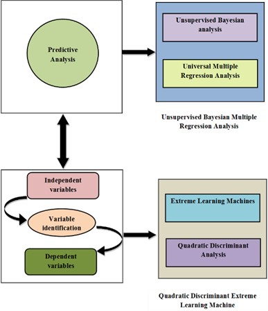
Fig. 1 displays the analysis of independent variables for the assessment of environmental influences on radon levels. A novel approach, integrating Unsupervised Bayesian Multiple Regression Analysis which is the combination of Universal Multiple Regression Analysis and Unsupervised Bayesian Analysis addresses challenges in predicting indoor radon levels. Additionally, a Quadratic Discriminant Extreme Learning Machine is introduced for variable identification, which is a combination of Quadratic Discriminant Analysis and Extreme Learning Machine, handling Non-Gaussian residual distributions and enhancing predictive accuracy. This comprehensive methodology produces resilient models capable of precisely estimating indoor radon levels and identifying influential factors in air pollution studies. The following section will include further details on this method.
3.1. Unsupervised Bayesian multiple regression analysis
Unsupervised Bayesian Multiple Regression Analysis is a novel approach which introduced for the predictive analysis problem to address the issue of radon concentration due to the complex interactions between several factors, including different house surroundings, ventilation systems, etc. to determine the precise impacts of each predictor variable separately, therefore Unsupervised Bayesian Multiple Regression Analysis has been implemented to solve the predictive analysis problem. The proposed approach was the combination of two existing techniques namely Unsupervised Bayesian analysis and Universal multiple regression analysis which will be explained detailed in below.
Unsupervised Bayesian analysis is a statistical technique used to analyze data without labeled outcomes. It involves incorporating existing information or assumptions about relationships among variables, such as correlations between factors. The goal of unsupervised learning is to identify hidden patterns or structures in the data without predefined labels or instructions. Bayesian analysis updates probabilities as new data is observed, refining the understanding of the data over time. It also manages uncertainty by providing a range of probable values, allowing for better understanding of predictions and conclusions. The Bayes Theorem is the core of Bayesian analysis, which mathematically combines prior information with new data to update the probability of a hypothesis. Bayesian methods are well-suited for managing complex data interactions, as they model these interactions more accurately than traditional methods. Furthermore, by incorporating prior knowledge and updating probabilities with new data, Bayesian analysis becomes more robust, providing reliable results even in complex and noisy data. It connects the posterior distribution of the parameters to the prior distribution of the parameters and the probabilities of the data given the parameters , which shown in Eq. (1):
The combination of the probabilities and parameter priors yields the posterior for a specific model, which implemented in both batch and online versions, which shown in Eq. (2) and Eq. (3):
Eq. (2) refers to batch processing which handling data in large sets, often all at once, and is well-suited for offline analysis scenarios where the complete dataset is accessible for processing:
Eq. (3) refers to online processing which involves the incremental handling of data, either in real-time or in small batches, which is ideal for scenarios involving streaming or continuous data streams.
Batch processing and Online processing aims to compute the predictive posterior distribution by combining prior knowledge and updating probabilities given in Eq. (4):
where: is the posterior distribution, representing the updated beliefs about the parameters given the observed data ; is the probability, indicating the probability of observing the data given a particular set of parameters ; is the prior distribution, representing the prior beliefs about the parameters before observing the data; is the marginal probability, serving as a normalizing constant ensuring that the posterior distribution integrates to 1; data set , and a model m with parameters ; prior over model parameters: ; probability of model parameters for data set ; prior over model class: .
A posterior distribution representing updated views about the parameters, given the observed data is the output of Unsupervised Bayesian analysis. According to Bayes’ Theorem, this posterior distribution captures the integration of prior beliefs with the probabilities of the data given the parameters The posterior distribution offers a thorough and current understanding of the underlying parameters by combining the information from previous studies with the new signal found in the data. The foundation of Bayesian inference is this integration process, which allows for a methodical approach to revealing hidden structures, patterns, or parameters in unsupervised learning settings. Moreover, this output provides better to Universal multiple regression analysis which is explained below.
Furthermore, Universal multiple regression analysis aims to represent the connection between one independent variable and one dependent variable. It is an extension of the notion of basic linear regression. It utilizes multiple explanatory factors to predict the value of a response variable, thereby enhancing predictive power, especially crucial in navigating the complexities of air pollution studies where numerous variables influence indoor radon levels. By modeling the linear connections between multiple explanatory factors and the response variable, it captures intricate real-world relationships essential for accurate predictions. This method extends ordinary least-squares regression to incorporate multiple predictors, providing flexibility in analyzing air pollution data and adapting to intricate complexities. Additionally, it offers quantitative assessments of each variable's contribution to the variance in indoor radon levels, facilitating informed decision-making and prioritizing interventions. Its robustness to multicollinearity ensures reliable coefficient estimates even with highly correlated predictor variables, enhancing model reliability. An equation for multiple linear regression takes the following generic form in Eq (5):
where: is the dependent variable (e.g., indoor radon concentration); is the intercept; , ,…, are the coefficients for the independent variables , ,…, ; is the error term.
The output of universal multiple regression analysis is a predictive model represented by Eq. (5), where the coefficients are determined based on the observed data. This model provides predictions for the dependent variable (e.g., indoor radon concentration) using the values of the independent variables . The output of universal multiple regression analysis improves predictive analysis by providing a robust model that considers multiple factors, offers insights into variable contributions.
Unsupervised Bayesian Multiple Regression Analysis combines the strengths of unsupervised Bayesian analysis and universal multiple regression. It enhances predictive analysis by providing insights into the contributions of each independent variable, reducing uncertainty in parameter estimate. This approach combines the modeling capabilities of universal multiple regression with the probabilistic output of unsupervised Bayesian analysis, addressing challenges in predictive analysis. The outcome is a sophisticated prediction model that considers uncertainties, combines prior information, and raises an intricate understanding of data correlations. This comprehensive approach produces a powerful tool for predictive modeling, offering robust solutions to complex analytical problems by computing the posterior distribution of the regression coefficients and the error term given the observed data and the model given as Eq. (6):
where, is the posterior distribution of the regression coefficients and the error term given the observed data , the independent variables , the observed data , and the model ; is the probability function representing the probability of observing the dependent variable ; is the prior distribution representing the regression coefficients and the error term before observing the data and the model ; is the marginal probabilities representing the probability of observing the data given the independent variables , the observed data , and the model .
This combines the prior knowledge and updating probabilities using Bayes theorem to obtain the posterior distribution, which represents the updated beliefs about the regression coefficients and the error term after observing the data.
Algorithm 1 displays the pseudocode of Unsupervised Bayesian Multiple Regression Analysis.
Algorithm 1: Unsupervised Bayesian Multiple Regression Analysis.
Input:
A dataset with observations of the dependent variable and multiple independent variables .
Output:
Coefficients representing the linear relationship between the dependent variable and independent variables.
Procedure:
Step 1-Initialize Prior for Bayesian Analysis:
Set initial beliefs about the distribution of parameters based on prior knowledge (prior distribution).
Step 2-Universal Multiple Regression Analysis:
Utilize the provided algorithm for Universal Multiple Regression Analysis using the training data to obtain coefficients .
Step 3- Probability Calculation:
Assess the probability of observing the data given the parameters using the obtained coefficients from the regression analysis.
Step 4-Prior and Probability Combination:
Combine the prior distribution and probabilities to obtain the unnormalized posterior distribution.
Step 5-Normalization:
Normalize the unnormalized posterior distribution to obtain the posterior distribution.
Step 6-Update Beliefs:
Use the posterior distribution as the updated beliefs about the parameters.
End
Fig. 2Flowchart of unsupervised Bayesian multiple regression analysis
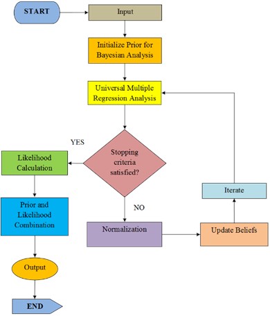
The benefits of both universal multiple regression analysis and unsupervised Bayesian analysis are combined in the Unsupervised Bayesian Multiple Regression Analysis method. It accepts previous knowledge about parameter distributions and training data with observations of dependent and independent variables as input. The approach first initializes the regression coefficients, then iteratively optimizes them by adding observed data and use Bayesian analysis to modify them. A probabilistic representation of the parameters is the result, which offers a more complex understanding of the correlations between the variables. Through the integration of Bayesian ideas into the multiple regression framework, this hybrid technique improves predictive modeling. Fig. 2 describes the flowchart of Unsupervised Bayesian Multiple Regression Analysis.
The flowchart illustrates the Unsupervised Bayesian Multiple Regression Analysis algorithm. It begins by inputting training data and prior beliefs. The algorithm initializes prior beliefs for Bayesian analysis and applies the Universal Multiple Regression Analysis to obtain initial coefficients. probability is calculated, and the prior and probabilities are combined to create the unnormalized posterior distribution, which is then normalized. The updated beliefs are derived, and the algorithm outputs both the posterior distribution and the final regression coefficients, offering a comprehensive probabilistic model. In addition, the output of the Unsupervised Bayesian Multiple Regression Analysis method solves the variable identification problem by utilizing "Quadratic Discriminant Extreme Learning Machine". Further details are provided in the next section.
3.2. Quadratic discriminant extreme learning machine
Quadratic Discriminant Extreme Learning Machine is a novel approach which implemented for the variable identification problem due to the intricacy of the residual distribution makes it more difficult to identify the variables affecting indoor radon levels. The variable identification problem has therefore been addressed with the introduction of the Quadratic Discriminant Extreme Learning Machine. The proposed approach combined two approaches quadratic discriminant analysis and the Extreme Learning Machine, which are described in more depth as follows.
Extreme Learning Machines (ELM) is a type of feedforward neural network used for tasks such as classifications and regression. The unique aspect of ELM is its ability to compute the output layer’s weights using a generalized inverse of the hidden layers output matrix. In this approach, ELM effectively handles Non-Gaussian residual distributions and provide more accurate predictions of indoor radon levels. Their strength lies in random input weight initialization and analytical output weight solutions. This approach enhances prediction accuracy, enabling ELMs to adapt to complex relationships within the data, especially when dealing with residuals that deviate from Gaussian distributions in indoor radon level predictions.
The output of ELM is calculated as follows given in Eq. (7):
where: is the output layer vector; is the weight vector between the hidden layer and the output layer; is the hidden layer output matrix.
The Hidden Layer Output Matrix () is calculated as follows given in Eq. (8):
where: is the activation function; is the weight vector between input and hidden layer; is the input vector; is the bias vector.
The following provides a thorough argument for the existing method:
A learning framework for single hidden layer feed forward neural networks (SLFN) is called Extreme Learning Machines. Extreme Learning Machines work on the general principle of generating connection weights at random between the input and hidden layers, then analytically computing the weights connecting the hidden layer to the output layer.
The architecture of Extreme Learning Machines is seen in Fig. 3. The hidden layer, which has a variable number of nodes depending on the issue, comes after the input layer, which is the signal source node. The transformation function of the hidden layer is based on the attenuation of a nonnegative linear function and its radial basis. In response to the input pattern, the hidden layer modifies activation function parameters and learning speed more slowly, whereas the output layer modifies linear weight and learning speed more quickly. Eq. (9) is a mathematical representation of neurons in the buried layer:
where is the threshold of the th hidden neuron, and is its value. The weight vector is what links the input neurons with the th hidden neuron. Let is the weight vector that joins the output neurons to the th hidden neuron.
Fig. 3Architecture of extreme learning machines
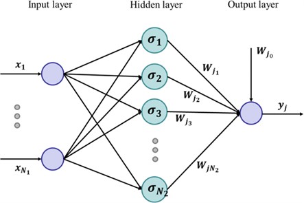
The output of Extreme Learning Machines is a trained neural network model with optimized connection weights between the input and hidden layers, as well as the analytically computed weights connecting the hidden layer to the output layer. In the context of the provided mathematical representation (Eq. (9)), the output involves the modified activation function parameters and learning speeds in the hidden layer, and the linear weights and learning speeds in the output layer. This output improves variable identification in indoor radon levels by efficiently capturing nonlinear patterns, adapting to data complexity, and providing optimized connections. The output of Extreme Learning Machines is given to quadratic discriminant analysis which explained as follows.
Moreover, each class in quadratic discriminant analysis is given a quadratic decision boundary, which allows for more flexibility when modeling complex interactions between predictors and response variables. Quadratic Discriminant Analysis is appropriate in scenarios where linear bounds, as in Linear Discriminant Analysis, are insufficient to appropriately reflect the underlying relationships because it permits a more intricate depiction of class distributions, which allows for the accommodation of complicated data patterns. The following provides a thorough argument of Quadratic Discriminant Analysis method:
Compared to Linear Discriminant Analysis, Quadratic Discriminant Analysis handles different covariance matrices for each class, which makes it flexible enough to handle situations when there are different variances across classes. Because of its adaptability, Quadratic Discriminant Analysis more effectively represents the intricate and non-linear decision boundaries that are observed in datasets with a variety of class features. The benefit of using Quadratic Discriminant Analysis is that, as opposed to linear decision boundaries, it produces a first class decision boundary by being less stringent and accepting varying covariance matrix characteristics for different classes. A single-variable statistical technique called quadratic discriminant analysis has been used to build an algorithm based on the groups that reveal the agents or influencing layers that are visible. For class , the discriminant function is represented as follows as in Eq. (10):
where: is the vector of environmental parameters, is the covariance matrix for class; is the mean vector for class; is the prior probability of class.
The output of the discriminant function in quadratic discriminant analysis is . It is a metric that utilized for classifying observations into several groups. More specifically, the above Eq. (8) is used to construct the discriminant function for each class . Next, the most likely class for a particular input vector is projected to be the one with the greatest discriminant function value. This output contributes to solving the variable identification problem by the discriminant function in Quantitative Discriminant Analysis involves coefficients that are associated with each environmental parameter (variable). These coefficients are derived from the mean vectors, covariance matrices, and prior probabilities of the different classes during the training phase.
The Quadratic Discriminant Extreme Learning Machine provides a useful method for identifying variables related to indoor radon levels. The combined result is a trained neural network that recognizes complex nonlinear patterns. To further improve variable identification, the Quadratic Discriminant Extreme Learning Machine also makes use of discriminant function coefficients from Quadratic Discriminant Analysis. By effectively addressing the intricacies of the data and maximizing the relationships between variables in the model, this all-encompassing method raises the accuracy of indoor radon level estimates. The pseudocode for the Quadratic Discriminant Extreme Learning Machine is shown in Algorithm 2.
Algorithm 2: Quadratic Discriminant Extreme Learning Machine.
Input:
Input data matrix of size , where is the number of samples and is the number of features.
Target class labels or output matrix of size where is the number of output nodes.
Number of classes,
Number of hidden nodes,
Output:
Output Weights of size
Bias vector of size
Class-specific mean vectors ( 1 to ).
Class-specific covariance matrices ( 1 to ).
Class priors ( 1 to ).
Algorithm Steps:
Step 1 –Apply Quadratic Discriminant Analysis (QDA):
a) For each class ( 1 to ):
i. Calculate the class-specific mean vector
ii. Calculate the class-specific covariance matrix
iii. Calculate the class prior probability
Step 2 –Initialize Extreme Learning Machine (ELM):
a) Randomly initialize input weights ( 1 to ) and biases ( 1 to ) connecting input layer to hidden layer.
Step 3 –Calculate ELM hidden layer output matrix using QDA parameters:
a) For each hidden node ( 1 to ):
i. Calculate activation using QDA mean vectors and covariance matrices: for each hidden node.
Step 4 –Compute the ELM output weights and bias using the following equation:
a) where pinv denotes the pseudo-inverse.
b) Bias can be calculated for better fitting.
End
The Quadratic Discriminant Extreme Learning Machine algorithm combines the discriminative power of Quadratic Discriminant Analysis with the flexibility of Extreme Learning Machine to optimize weights and biases. It utilizes Quadratic Discriminant Analysis’s class-specific statistics to enhance ELM’s ability to capture nonlinear patterns, resulting in improved variable identification and accurate predictions for multi-class classification tasks. Fig. 4 represents the flowchart of Quadratic Discriminant Extreme Learning Machine for Radon Prediction.
Fig. 4Flowchart of quadratic discriminant extreme learning machine for radon prediction
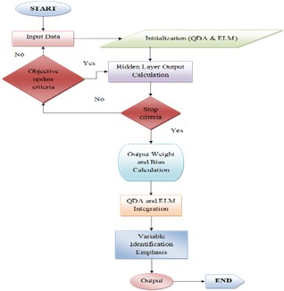
The data processing process depicted in the flowchart starts with the input data, initializes Quadratic Discriminant Analysis and ELM components, looks for objective update criteria, computes output from a hidden layer, determines when to stop, computes output weight and biases, integrates QDA and ELM components, stresses variable identification, and outputs the intended outcome in the end. Because the process is data-driven, each step's goal must be determined within a certain context or domain. The “END” label marks the end of the flowchart.
Overall, the proposed approach integrates Unsupervised Bayesian Multiple Regression Analysis with a Quadratic Discriminant Extreme Learning Machine for comprehensive indoor radon level predictions. It utilizes Unsupervised Bayesian Multiple Regression Analysis for predictive analysis in radon concentration, which combines universal multiple regression and unsupervised Bayesian analysis for linear relationships. Then, it makes use of a Quadratic Discriminant Extreme Learning Machine for variable identification in indoor radon levels, which combines the Quadratic Discriminant Analysis and Extreme Learning Machines for efficient handling of nonlinear patterns. This synergistic method enhances variable identification, providing a sophisticated predictive model that considers uncertainties and complex correlations in the data. The algorithm combines statistical and machine learning techniques for robust indoor radon level predictions, addressing multifaceted interactions. Section 4 will describe the performance and comparison of the proposed technique.
4. Results and discussion
The proposed approach for predictive analysis and variable identification is examined in this section, with particular attention focused to dependent and independent variables. It looks at the performance of the Unsupervised Bayesian Multiple Regression Analysis and Quadratic Discriminant Extreme Learning Machine method.
4.1. Experimental setup
Every home’s radon gas concentration is determined using a dosimeter that was created by BARC Mumbai. The dosimeter is maintained one meter above the ground, and measurements are taken in the summer, winter, and rainy seasons.
Tool used: Tableau Desktop; OS: Windows 10 home; Processor: Intel (R) Core (TM) i5-8265U CPU@1.60 GHZ 1.80 GHZ; RAM: 16 .00 GB.
4.2. Dataset description
Three different seasons were observed at the Dadar, Mumbai location: the rainy season (June to September), the winter season (October to January), and the summer season (February to May). The measured values of radon concentrations were used to calculate the Pearson Correlation Coefficient for three environmental parameters: temperature, humidity, and atmospheric pressure. Table 2 summarizes the Pearson correlation matrix for radon and climatic parameter.
Table 2Pearson correlation matrix for radon and climatic parameter
Season | Temp [°C] | Humidity % | Pressure kPa |
Rainy | 0.1591 | 0.128 | 0.107 |
Winter | 0.208 | 0.189 | 0.152 |
Summer | 0.233 | 0.402 | 0.234 |
There is no discernible relationship between environmental parameters and radon concentration at the Dadar, Mumbai, Maharashtra location. However, Table 2 shows that during the summer, humidity had a recorded influence of 0.402, while for other parameters, the correlation coefficient in absolute value is less than 0.25 during the rainy, winter, and summer seasons.
4.3. Experimental results
Tableau was used for data analysis and simulation, with both independent and dependent variables (such as temperature, humidity, and air pressure) as input. A differential equation was used to compute the integrated radon concentration, which was then compared to the measured value. There were not many variations between the calculated and observed values, according to the study. As a result, it concluded that temperature, humidity, and air pressure have a negligible effect on the integrated radon concentration that was computed because of the differential equation that was used in the simulation.
4.4. Performance analysis of the proposed method
This integrated predictive analysis and variable identification approach is evaluated using key indicators such as air pressure and radon content. It also evaluates how well Unsupervised Bayesian Multiple Regression Analysis enhances predictive analysis and detects diseases caused by radon concentrations. It is evaluated how well Quadratic Discriminant Extreme Learning Machine identify specific variables identification.
The link between temperature and radon concentration is seen in Fig. 5. The graph shows that the value of the radon concentration is roughly proportionate to the floor-by-floor temperature. With a correlation coefficient of 0.159, the temperature during the rainy season is positively and inversely correlated. The multiple regression equation for the measurement at the Dadar Mumbai site during the rainy season was computed using the following parameters: temp and correlation coefficient, 0.159 in Eq. (11):
Fig. 5Plotting a regression path between temperature and radon levels during the rainy season in a scattering diagram
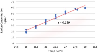
Fig. 6A scattering diagram showing the direction of the plotted relationship between the wintertime temperature and radon concentration
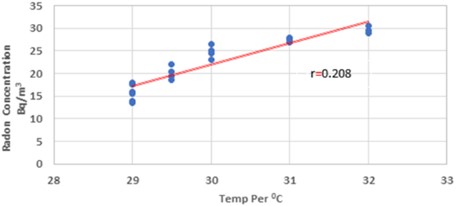
Fig. 6 indicates that there is a negative relationship between the two variables. The presented graph demonstrates that the value of the indoor radon concentration is directly correlated with the floor-wise temperature. The winter temperature has a slight correlation with the correlation coefficient of 0.208. Eq. (12) presents the multiple regression equation that was developed for the measurement at Dadar Mumbai location during the winter season, taking into account the parameters temp and 0.208:
Fig. 7 indicates a marginally favorable relationship between the two variables. With a correlation value of 0.233, it shows the direct proportionality of indoor radon concentration with temperature variations floor by floor during the summer. The multiple regression equation that was computed for the measurement at the Dadar Mumbai site during the summer season took into account the temperature and the correlation coefficient, 0.233, as indicated in Eq. (13):
Fig. 7A scattering diagram showing the direction of the plotted relationship between summertime temperature and radon concentration
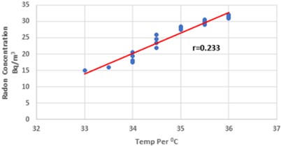
Fig. 8 indicates a marginally favorable relationship between the two variables. The plotted graph demonstrates that the relationship between the value of indoor radon concentration and humidity is direct. The correlation coefficient, which is 0.128, shows a modest relationship between humidity and the rainy season. The multiple regression equation for the measurement in Dadar, Mumbai, during the rainy season, taking into account the humidity and 0.128, is represented in Eq. (14):
Fig. 8Plotted regression direction between radon concentration and humidity during the rainy season is displayed in a scattering diagram
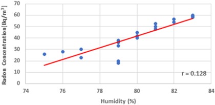
Fig. 9Plotted regression direction between wintertime humidity and radon levels on a scattering diagram
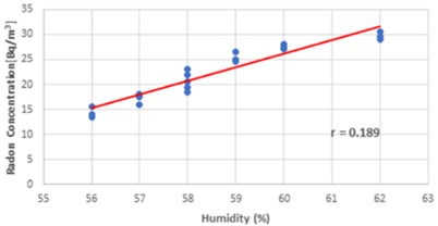
Examining the association between radon concentration and humidity levels is shown in Fig. 9. The above graph illustrates how indoor radon levels and humidity are directly correlated throughout the winter. Eq. (15) displays the multiple regression equation with humidity and 0.189 for the Dadar Mumbai area during the winter season:
There is a somewhat favorable association between humidity and radon concentration in the summer according to the scatter plot in Fig. 10. The graph’s red trend line indicates that radon concentration grows in tandem with increased humidity. The somewhat favorable association between greater humidity levels and enhanced radon concentrations is indicated by the correlation coefficient, 0.402 which shows in Eq. (16):
The link between air pressure and radon levels during the rainy season is shown in Fig. 11. This graph shows the straight proportionality between the independent variable, the atmospheric pressure during the rainy season, and the radon concentration. The regression Eq. (17) for pressure and radon concentration parameters in Dadar, Mumbai, during the rainy season has a correlation value of 0.107:
Fig. 10A scattering diagram showing the direction of the observed relationship between summertime humidity and radon concentration
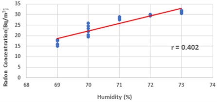
Fig. 11Plotted regression direction between pressure and radon concentration during the rainy season is displayed in a scattering diagram.

The -axis represents atmospheric pressure, while the -axis represents radon concentration. Fig. 12 illustrates the link between radon concentration and atmospheric pressure. This graph shows the straight proportionality between the independent variable, the atmospheric pressure during the winter, and the radon concentration. Eq. (18) displays the results of a multiple regression analysis using pressure and 0.152 for the Dadar Mumbai area during the winter season:
Fig. 12Plotted regression path between wintertime pressure and radon concentration on a scattering diagram
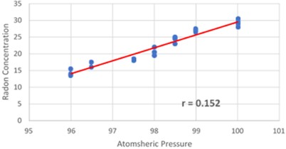
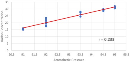
Fig. 13 illustrates the relationship between summertime air pressure and radon levels. The data points show that as air pressure increases from 90 to 95, there is a modest increase in radon concentration. The multiple regression equation for the parameters Pressure and Indoor Radon Concentration at location Dadar Mumbai in the summer, with 0.233, is displayed in Eq. (19):
Fig. 13Plotting a regression path between summertime pressure and radon concentration in a scattering diagram
4.5. Comparison method
This section, as noted in [29], contrasts the proposed approach's Mean Absolute Error (MAE), Root Mean Squared Error (RMSE), Root Mean Squared Logarithmic Error (RMSLE), Percentage Bias, and Coefficient of relation with the existing Inverse distance weighting, Empirical Bayesian Kriging, and Ordinary Kriging approaches. It illustrates how the proposed approach outperforms or is on trend with current methods in the variables identification and predictive analysis domains. A thorough analysis of these measures is used to achieve this. The comparison goes beyond performance metrics to include Percentage Bias and Coefficient of Relation to confirm the benefit or efficiency of the proposed strategy in managing diagnostics that enable a thorough comprehension of the radon concentration of predictive analysis and variable identification.
Fig. 14Comparison of MAE with existing methods
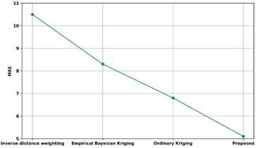
The comparison of the proposed model's MAE with that of other current methods is shown in Fig. 14. The MAE of the proposed method is contrasted with that of already available methods like Inverse distance weighting, Empirical Bayesian Kriging, and Ordinary Kriging approaches. The proposed model's MAE comes in at 5.1 %, whereas the MAE of Inverse distance weighting, Empirical Bayesian Kriging, and Ordinary Kriging approaches are, in that order, 10.5 %, 8.3 %, and 6.8 %. Thus, variable identification has improved due to the Quadratic Discriminant Extreme Learning Machine with low MAE.
Fig. 15Comparison of RMSE with existing methods
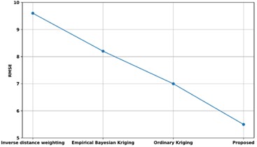
Fig. 15 displays a comparison of the RMSE of the proposed approach with those of other available techniques. The RMSE of the proposed approach is compared to those of existing techniques such as Ordinary Kriging approaches, Empirical Bayesian Kriging, and Inverse distance weighting. The RMSE of the proposed model is 5.5 %, while the RMSE of the techniques such as inverse distance weighting, empirical Bayesian kriging, and ordinary kriging are, respectively, 9.6 %, 8.2 %, and 7.0 %. Thus, the Unsupervised Bayesian Multiple Regression Analysis has enhanced predictive analysis with low RMSE.
Fig. 16Comparison of RMSLE with existing methods
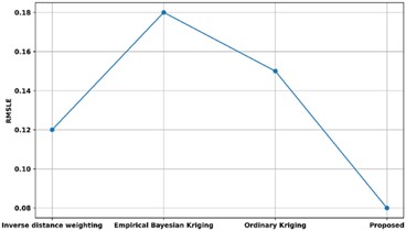
A comparison of the proposed approach’s RMSLE with other existing methodologies is shown in Fig. 16. The proposed method’s RMSLE is contrasted with that of other methods already in use, including inverse distance weighting, empirical Bayesian kriging, and ordinary kriging approaches. The proposed model's RMSLE is 0.08 %, whereas the RMSLE of methods utilizing inverse distance weighting, empirical Bayesian kriging, and conventional kriging are 0.12 %, 0.18 %, and 0.15 %, respectively. Thus, the use of machine learning in Quadratic Discriminant Extreme Learning Machine has enhanced variable identification with low RMSLE.
Fig. 17Comparison of percentage Bias with existing methods
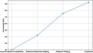
Fig. 17 displays a comparison of the Percentage Bias of the proposed methodology with various current approaches. The Percentage Bias of the proposed approach is compared with that of existing techniques, such as Inverse distance weighting, Empirical Bayesian Kriging, and Ordinary Kriging. The percentage bias of the proposed model is 92 %, while the percentage biases of approaches that use Inverse distance weighting, Empirical Bayesian Kriging, and Ordinary Kriging are, respectively, 20 %, 42 %, and 76 %. Thus, the Unsupervised Bayesian Multiple Regression Analysis has enhanced predictive analysis with high Percentage Bias.
A comparison of the proposed methodology’s coefficient of relation with many other existing methods is shown in Fig 18. The proposed method’s coefficient of relation is contrasted with that of other methods now in use, including Inverse distance weighting, Empirical Bayesian Kriging, and Ordinary Kriging approaches. The proposed model’s correlation coefficient is 81, compared to the correlation coefficients of models utilizing Inverse distance weighting, Empirical Bayesian Kriging, and Ordinary Kriging, which are 24, 48, and 66, respectively. Thus, the Unsupervised Bayesian Multiple Regression Analysis has enhanced predictive analysis with high Coefficient of relation.
Fig. 18Comparison of coefficient of relation with existing methods
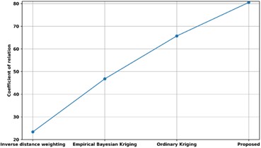
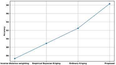
Fig. 19 shows a comparison of the accuracy of the proposed technique with several different methods already in use. The accuracy of the proposed method is compared with existing approaches such as Ordinary Kriging, Empirical Bayesian Kriging, and Inverse distance weighting. The accuracy of the proposed model is 98.2 %, whereas the models that use Ordinary Kriging, Empirical Bayesian Kriging, and Inverse distance weighting have corresponding accuracy of 92.5 %, 89 %, and 85 %. Predictive analysis has therefore been improved by Unsupervised Bayesian Multiple Regression Analysis with accuracy rate.
Fig. 19Comparison of accuracy with existing methods
A comparison of the precision of the proposed approach with several existing methods is presented in Fig. 20. The precision of the proposed technique is contrasted with current methodologies like Inverse Distance Weighting, Ordinary Kriging, and Empirical Bayesian Kriging. The proposed model’s precision is 96.3 %, whereas the models that employ inverse distance weighting, ordinary kriging, and empirical Bayesian kriging have respective precisions of 91.7 %, 89.5 %, and 86.4 %. Thus, Unsupervised Bayesian Multiple Regression Analysis has enhanced predictive analysis with high precision rate.
Fig. 20Comparison of precision with existing methods
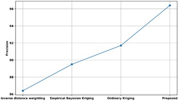
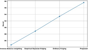
Fig. 21 compares the recall of the proposed approach with several other approaches that are currently in use. The proposed technique’s recall is compared to existing approaches such as Empirical Bayesian Kriging, Ordinary Kriging, and Inverse Distance Weighting. The proposed model has a recall of 97.8 %, whereas the models using conventional kriging, empirical Bayesian kriging, and inverse distance weighting had recalls of 84.7 %, 88.9 %, and 93.4 %, respectively. Thus, variable identification has improved due to the Quadratic Discriminant Extreme Learning Machine with high recall.
Fig. 21Comparison of recall with existing methods
The sensitivity of the proposed method is contrasted with many alternative ways that are currently in use in Fig. 22. The sensitivity of the proposed method is contrasted with that of other methods that are already in use, including Inverse Distance Weighting, Ordinary Kriging, and Empirical Bayesian Kriging. The models using conventional kriging, empirical Bayesian kriging, and inverse distance weighting have recalls of 95 %, 92 %, and 95 %, respectively, whereas the recommended model had a sensitivity of 96 %. Thus, Unsupervised Bayesian Multiple Regression Analysis has enhanced predictive analysis with high sensitivity rate.
Fig. 22Comparison of sensitivity with existing methods
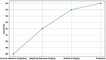
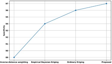
Fig. 23 compares the specificity of the proposed approach with several other approaches that are currently in use. The proposed method’s specificity is compared to that of existing approaches, such as Empirical Bayesian Kriging, Ordinary Kriging, and Inverse Distance Weighting. The proposed approach has a sensitivity of 97 %, while the models utilizing inverse distance weighting, conventional kriging, and empirical Bayesian kriging have specificities of 96 %, 94 %, and 89 %, respectively. Thus, variable identification has improved due to the Quadratic Discriminant Extreme Learning Machine with high specificity.
Fig. 23Comparison of specificity with existing methods
Simple linear regression is a powerful mathematical algorithm that excels under certain conditions due to its simplicity, efficiency, and interpretability. It models the relationship between two variables with a straight line, making it easy to understand and communicate findings. It is computationally efficient, requiring only two parameters, making it suitable for large datasets. Its ease of implementation is enhanced by built-in functions in software packages and programming languages.
Overall the comparison method in predictive analysis and variable identification evaluates the proposed approach against existing methods using various performance metrics. These include MAE, RMSE, RMSLE, Percentage Bias, Coefficient of Relation, Accuracy, Precision, Recall, sensitivity and specificity. The proposed approach outperforms or aligns with current methods in these domains with a Percentage Bias of 92 %, and Coefficient of relation with 81. Additionally, the approach achieves an impressive 5.1 % of MAE, 5.5 % of RMSE, 0.08 % of RMSLE establishing it as a superior option for predictive analysis and variable identification in radon concentration. This advantage over Inverse distance weighting, Empirical Bayesian Kriging, and Ordinary Kriging techniques is particularly notable in real-world circumstances with complicated dynamics and interference difficulties.
5. Conclusions
Particularly in the complex field of air pollution research, where various hypotheses needed for careful evaluation and careful interpretation, regression analysis was essential for prediction and variable identification. The proposed method Unsupervised Bayesian Multiple Regression Analysis was used for predictive analysis and this technique solved the multicollinearity problems in estimating indoor radon levels and it accurately provided the individual effects of each predictor variable by taking into account the intricate relationships between the many components involved in the prediction of radon levels inside. Furthermore, the proposed Quadratic Discriminant Extreme Learning Machine was used for variable identification and it solved the indoor radon levels issues affected by complex residual distributions, and it developed models that were more resistant to non-Gaussian residual distributions more capable of accurately identifying the variables influencing indoor radon levels. When compared to Inverse distance weighting, Empirical Bayesian Kriging, and Ordinary Kriging methods, the comparative analysis provides an unqualified demonstration of the method's superiority, exhibiting remarkable performance metrics like 5.5 % of RMSE, 92 % of Percentage Bias, 81 of Coefficient of relation, 98.2 % of accuracy, 96.3 % of precision and 96 % of sensitivity by the proposed technique Unsupervised Bayesian Multiple Regression Analysis, which solved the predictive analysis problems in radon concentration. Also, achieved 5.1 % of MAE, 0.08 % of RMSLE, 97.8 % of recall and 97 % of specificity by the proposed technique of Quadratic Discriminant Extreme Learning Machine which used for variable identification in radon concentration. This all-encompassing method promises sensitive operational efficiency and is a significant advancement in variable identification and predictive analysis in real-world scenarios. It represents a significant advance in this knowledge of radon concentrations and has the potential to revolutionize this sector.
References
-
N. A. Uyanik, Z. Öncü, O. Uyanik, and I. Akkurt, “Determination of natural radioactivity from 232Th with Gamma-ray spectrometer in Dereköy-Yazır (Southwestern Anatolia),” Acta Physica Polonica A, Vol. 128, No. 2B, pp. B–441-B-443, Aug. 2015, https://doi.org/10.12693/aphyspola.128.b-441
-
H. Zeeb and F. Shannoun, WHO Handbook on Indoor Radon: a Public Health Perspective. Geneva: WHO Press, 2009.
-
D. J. Steck, “Annual average indoor radon variations over two decades,” Health Physics, Vol. 96, No. 1, pp. 37–47, Jan. 2009, https://doi.org/10.1097/01.hp.0000326449.27077.3c
-
C. Coletti et al., “The assessment of local geological factors for the construction of a geogenic radon potential map using regression kriging. a case study from the Euganean Hills volcanic district (Italy),” Science of The Total Environment, Vol. 808, p. 152064, Feb. 2022, https://doi.org/10.1016/j.scitotenv.2021.152064
-
M. Hosoda, S. Tokonami, T. Suzuki, and M. Janik, “Machine learning as a tool for analysing the impact of environmental parameters on the radon exhalation rate from soil,” Radiation Measurements, Vol. 138, p. 106402, Nov. 2020, https://doi.org/10.1016/j.radmeas.2020.106402
-
J. Elío, E. Petermann, P. Bossew, and M. Janik, “Machine learning in environmental radon science,” Applied Radiation and Isotopes, Vol. 194, p. 110684, Apr. 2023, https://doi.org/10.1016/j.apradiso.2023.110684
-
D. Dai, “Neighborhood characteristics of low radon testing activities: a longitudinal study in Atlanta, Georgia, United States,” Science of The Total Environment, Vol. 834, p. 155290, Aug. 2022, https://doi.org/10.1016/j.scitotenv.2022.155290
-
J. Moon and H. Yoo, “Residential radon exposure and leukemia: a meta-analysis and dose-response meta-analyses for ecological, case-control, and cohort studies,” Environmental Research, Vol. 202, p. 111714, Nov. 2021, https://doi.org/10.1016/j.envres.2021.111714
-
A. Ruano-Ravina et al., “Indoor radon exposure and COPD, synergic association? A multicentric, hospital-based case-control study in a radon-prone area,” Archivos de Bronconeumología (English Edition), Vol. 57, No. 10, pp. 630–636, Oct. 2021, https://doi.org/10.1016/j.arbr.2020.11.020
-
A. M. Hussein, K. O. Abdullah, A. H. Fattah, and R. R. Mohammed-Ali, “Estimating atmospheric radon deviation using statistical coefficients: Sulaymaniyah city, Iraq, as a case of study,” Isotopes in Environmental and Health Studies, Vol. 59, No. 2, pp. 202–215, Mar. 2023, https://doi.org/10.1080/10256016.2023.2195175
-
L. Martin-Gisbert et al., “Radon exposure and its influencing factors across 3,140 workplaces in Spain,” Environmental Research, Vol. 239, p. 117305, Dec. 2023, https://doi.org/10.1016/j.envres.2023.117305
-
O. B. Akanbi, “Spatial analysis of soil radon gas concentration in Southwestern Nigeria: a Bayesian approach,” International Journal of Applied Science and Mathematics, Vol. 9, No. 3, pp. 36–46, 2022.
-
P. Vukotic, Z. Stojanovska, and N. Antovic, “Developing a method for predicting radon concentrations above a reference level in new montenegrin buildings,” Journal of Environmental Radioactivity, Vol. 227, p. 106500, Feb. 2021, https://doi.org/10.1016/j.jenvrad.2020.106500
-
P. Nojarov, P. Stefanov, and K. Turek, “Influence of some climatic elements on radon concentration in Saeva Dupka Cave, Bulgaria,” International Journal of Speleology, Vol. 49, No. 3, pp. 235–248, Sep. 2020, https://doi.org/10.5038/1827-806x.49.3.2349
-
J. Cerqueiro-Pequeño, A. Comesaña-Campos, M. Casal-Guisande, and J.-B. Bouza-Rodríguez, “Design and development of a new methodology based on expert systems applied to the prevention of indoor radon gas exposition risks,” International Journal of Environmental Research and Public Health, Vol. 18, No. 1, p. 269, Dec. 2020, https://doi.org/10.3390/ijerph18010269
-
M. Lorenzo-Gonzalez et al., “Lung cancer risk and residential radon exposure: A pooling of case-control studies in northwestern Spain,” Environmental Research, Vol. 189, p. 109968, Oct. 2020, https://doi.org/10.1016/j.envres.2020.109968
-
Rodríguez-Martínez et al., “Residential radon and small cell lung cancer. Final results of the small cell study,” Archivos de Bronconeumología, Vol. 58, No. 7, pp. 542–546, Jul. 2022, https://doi.org/10.1016/j.arbres.2021.01.027
-
K. F. Al-Shboul, “Unraveling the complex interplay between soil characteristics and radon surface exhalation rates through machine learning models and multivariate analysis,” Environmental Pollution, Vol. 336, p. 122440, Nov. 2023, https://doi.org/10.1016/j.envpol.2023.122440
-
C. Seyis, S. Inan, and M. N. Yalçın, “Major factors affecting soil radon emanation,” Natural Hazards, Vol. 114, No. 2, pp. 2139–2162, Jul. 2022, https://doi.org/10.1007/s11069-022-05464-y
-
H. Y. Joo, J. W. Kim, S. Y. Jeong, Y. S. Kim, and J. H. Moon, “Use of big data for estimation of impacts of meteorological variables on environmental radiation dose on Ulleung Island, Republic of Korea,” Nuclear Engineering and Technology, Vol. 53, No. 12, pp. 4189–4200, Dec. 2021, https://doi.org/10.1016/j.net.2021.07.001
-
E. Benà et al., “A new perspective in radon risk assessment: mapping the geological hazard as a first step to define the collective radon risk exposure,” Science of The Total Environment, Vol. 912, p. 169569, Feb. 2024, https://doi.org/10.1016/j.scitotenv.2023.169569
-
T. Haider et al., “Identification of radon anomalies induced by earthquake activity using intelligent systems,” Journal of Geochemical Exploration, Vol. 222, p. 106709, Mar. 2021, https://doi.org/10.1016/j.gexplo.2020.106709
-
M. Panahi et al., “Spatial modeling of radon potential mapping using deep learning algorithms,” Geocarto International, Vol. 37, No. 25, pp. 9560–9582, Dec. 2022, https://doi.org/10.1080/10106049.2021.2022011
-
S. Zhang, Z. Shi, G. Wang, R. Yan, and Z. Zhang, “Groundwater radon precursor anomalies identification by decision tree method,” Applied Geochemistry, Vol. 121, p. 104696, Oct. 2020, https://doi.org/10.1016/j.apgeochem.2020.104696
-
J. Pirkkanen et al., “A research environment 2 km deep-underground impacts embryonic development in lake whitefish (Coregonus clupeaformis),” Frontiers in Earth Science, Vol. 8, p. 327, Jul. 2020, https://doi.org/10.3389/feart.2020.00327
-
L. Li et al., “A spatiotemporal ensemble model to predict gross beta particulate radioactivity across the contiguous United States,” Environment International, Vol. 156, p. 106643, Nov. 2021, https://doi.org/10.1016/j.envint.2021.106643
-
E. A. Njoku and D. E. Tenenbaum, “Quantitative assessment of the relationship between land use/land cover (LULC), topographic elevation and land surface temperature (LST) in Ilorin, Nigeria,” Remote Sensing Applications: Society and Environment, Vol. 27, p. 100780, Aug. 2022, https://doi.org/10.1016/j.rsase.2022.100780
-
M. Adelikhah, A. Shahrokhi, M. Imani, S. Chalupnik, and T. Kovács, “Radiological assessment of indoor radon and thoron concentrations and indoor radon map of dwellings in Mashhad, Iran,” International Journal of Environmental Research and Public Health, Vol. 18, No. 1, p. 141, Dec. 2020, https://doi.org/10.3390/ijerph18010141
Cited by
About this article

The authors have not disclosed any funding.
The datasets generated during and/or analyzed during the current study are available from the corresponding author on reasonable request.
Anil Pawade worked on modelling, preparing and writing draft, analysis and generating proper images. Shrikant Charhate worked on draft review and conceptualization, overall guidance.
The authors declare that they have no conflict of interest.
